Foraging toolkit demo - random foragers
Outline
Introduction
Users of the foraging toolkit are interested in analyzing animal movement data, with the goal of determining what factors contribute to each agent’s decisions of where to move.
Given either a simulation output or real-world measured location data, we would like to infer which factors influence the agents’ movement. In this notebook, we consider two possible factors: proximity to other agents, and closeness to food. Each factor has an associated score that is computed at each location where an agent might move. These scores are used as derived predictors in a statistical model of agents’ movements.
The fit coefficients of these derived predictor scores can be interpreted as how predictive each factor is of agents’ movement decisions.
For more details, see [1], in particular Fig.2.
To validate the methodology, this notebook uses the foraging toolkit to simulate movements of random foraging agents, moving in random directions with random step sizes (with some step distance preferences). Therefore, we expect that neither proximity nor food have any significant effect at the inference stage (i.e. the corresponding predictor coefficients should be close to zero).
[1] R. Urbaniak, M. Xie, and E. Mackevicius, “Linking cognitive strategy, neural mechanism, and movement statistics in group foraging behaviors,” Sci Rep, vol. 14, no. 1, p. 21770, Sep. 2024, doi: 10.1038/s41598-024-71931-0.
[1]:
# importing packages. See https://github.com/BasisResearch/collab-creatures for repo setup
import logging
import os
import random
import time
import dill
import matplotlib.pyplot as plt
import numpy as np
import plotly.io as pio
import pyro
from IPython.display import HTML
pio.renderers.default = "notebook"
import collab.foraging.toolkit as ft
from collab.foraging import random_hungry_followers as rhf
logging.basicConfig(format="%(message)s", level=logging.INFO)
# users can ignore smoke_test -- it's for automatic testing on GitHub,
# to make sure the notebook runs on future updates to the repository
smoke_test = "CI" in os.environ
num_svi_iters = 10 if smoke_test else 1000
num_samples = 10 if smoke_test else 1000
notebook_starts = time.time()
Simulation
The random_hungry_followers module, imported as rhf, lets us simulate different groups of agents foraging in a gridworld environment. The user can adjust how big the environment is, how many agents are in the group, how much food reward is present, etc. The probabilities argument controls the (unnormalized) probability of choosing a step of each size in [-max_step_size, max_step_size]. For further explanation of what each input parameter means, run help(rhf.RandomForagers).
Currently the step sizes are pre-defined to the range ![[-4,\dots,4]](../../_images/math/ab6f33c35739071e67acd129f3ebdcd843efc8c7.png) .
.
Simulation of Random Foragers
Initialization
Initialize the grid with a specified grid size.
Randomly place
num_rewardsrewards on the grid.Normalize the probabilities for forager step size.
Generate Random Paths
For each forager:
Generate random
xandycoordinates as the cumulative sum of centered random steps based on the initialized probabilities, for example:
forager_x = np.cumsum(np.random.choice(num_steps, num_frames, probabilities, replace=True)) + (grid_size / 2) forager_y = ... # same as for x
Ensure the coordinates stay within the grid bounds.
Update Rewards
At each frame, remove a reward if a forager is next to it, starting from that frame onward.
[2]:
random.seed(23)
np.random.seed(23)
num_frames = 5 if smoke_test else 50 # The number of frames in the simulation.
grid_size = 40 # The size of the grid representing the environment.
random_foragers_sim = rhf.RandomForagers(
grid_size=grid_size, # The size of the grid representing the environment.
probabilities=[
1,
2,
3,
2,
1,
2,
3,
2,
1,
], # (potentially unnormalized) probabilities for each step size in [-4..4]
num_foragers=3, # The number of (randomly moving) foragers.
num_frames=num_frames, # The number of frames in the simulation.
num_rewards=15, # The number of rewards initially in the environment.
# Will disappear as foragers grab them by being within the `grab_range`.
grab_range=3, # The range within which rewards can be grabbed.
)
# run a particular simulation with these parameters
random_foragers_sim()
# the results of the simulation are stored in `random_foragers_sim.foragersDF` DataFrame.
# each row contains the x and y coordinates of a forager at a particular time
random_foragers_sim.foragersDF.head()
[2]:
| x | y | time | forager | type | |
|---|---|---|---|---|---|
| 0 | 20.0 | 23.0 | 0 | 0 | random |
| 1 | 24.0 | 23.0 | 1 | 0 | random |
| 2 | 26.0 | 25.0 | 2 | 0 | random |
| 3 | 24.0 | 28.0 | 3 | 0 | random |
| 4 | 22.0 | 26.0 | 4 | 0 | random |
We can plot the generated trajectories using plot_trajectories(), passing the corresponding DataFrame.
[3]:
ft.plot_trajectories(random_foragers_sim.foragersDF, "Random Foragers")
plt.show()
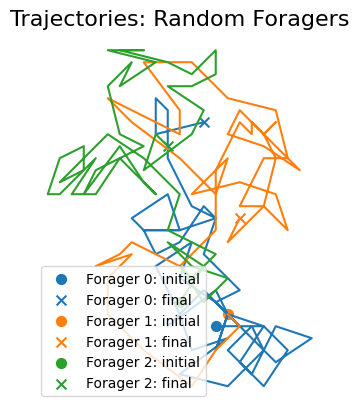
The foragers’ movements can be visualized using the animate_foragers() function.
[4]:
ft.animate_foragers(
random_foragers_sim, width=600, height=400, plot_rewards=True, point_size=6
)
Derived quantities
Suppose we observed this movement data from agents out in the world, and have several hypotheses for what may be contributing to the agents’ movement decisions. We’ll calculate derived predictor scores, which have high weight at locations/times where that hypothesis predicts that birds would want to go.
In practice, given the simulated data, we compute the values of the different derived quantities:
Predictors:
 for every forager
  at every timestep
  , giving the predicted expected future value of
  for forager
  at every grid point
  and time step
  .
.Scores:
 can be regarded as conditional probabilities of the forager
  ’s location at time
  , given the simulation state at time
  . This function has a peak at the actual location at time
  , and decays with distance from that point.
Note: as we shall see below, the values of  and
and  are evaluated only over the so-called local window
  corresponding to the immediate surroundings of forager
  at time
  (i.e. all the locations where it can possibly go).
In the remainder of this section we elaborate on how  and
and  are actually computed.
At the inference stage, we shall fit the scores to a linear combination of predictors with unknown coefficients. See Inference section below for more details.
Computation
The main function computing the predictors is derive_predictors_and_scores() (see documentation by help(ft.derive_predictors_and_scores))
[5]:
help(ft.derive_predictors_and_scores)
Help on function derive_predictors_and_scores in module collab.foraging.toolkit.derive:
derive_predictors_and_scores(foragers_object: collab.foraging.toolkit.utils.dataObject, local_windows_kwargs: Dict[str, Any], predictor_kwargs: Dict[str, Dict[str, Any]], score_kwargs: Dict[str, Dict[str, Any]], dropna: Optional[bool] = True, add_scaled_values: Optional[bool] = False) -> pandas.core.frame.DataFrame
A function that calculates a chosen set of predictors and scores for data by inferring their names from
keys in `predictor_kwargs` & `score_kwargs`, and dynamically calling the corresponding functions.
:param foragers_object: instance of dataObject class containing the trajectory data of foragers.
:param local_window_kwargs: dictionary of keyword arguments for `generate_local_windows` function.
:param predictor_kwargs: nested dictionary of keyword arguments for predictors to be computed.
Keys of predictor_kwargs set the name of the predictor to be computed.
The predictor name can have underscores, however, the substring before the first underscore must correspond
to the name of a predictor type in Collab. Thus, we can have multiple versions of the same predictor type
(with different parameters) by naming them as follows:
predictor_kwargs = {
"proximity_10" : {"optimal_dist":10, "decay":1, ...},
"proximity_20" : {"optimal_dist":20, "decay":2, ...},
"proximity_w_constraint" : {...,"interaction_constraint" : constraint_function,
"interaction_constraint_params": {...}}
}
:param score_kwargs: nested dictionary of keyword arguments for outcome variables
("scores") to be computed. The substring before the first underscore in dictionary keys must
correspond to the name of a score type in Collab, same as in `predictor_kwargs`
score_kwargs = {
"nextStep_linear" : {"nonlinearity_exponent" : 1},
"nextStep_squared" : {"nonlinearity_exponent" : 2},
}
:param dropna: set to `True` to drop NaN elements from the final DataFrame
:param add_scaled_values: set to `True` to compute scaled predictor scores
and add them as additional columns in final DataFrame
:return: final, flattened DataFrame containing all computed predictors as columns
The local windows  , where
 ![\mathfrak{G}:=[0:\textrm{grid size}-1]^2](../../_images/math/fae758bda80fb6543e1022b7fe0b4e532a0fa59b.png) is the entire computational grid, are used to compute the predictors and the scores over. A local window is generated for each forager
is the entire computational grid, are used to compute the predictors and the scores over. A local window is generated for each forager  at every time step
  , and it consists of all the grid points where forager
  can possibly go at step
  . To generate all the local windows for the simulation, use
generate_local_windows() method.
[6]:
help(ft.local_windows.generate_local_windows)
Help on function generate_local_windows in module collab.foraging.toolkit.local_windows:
generate_local_windows(foragers_object: collab.foraging.toolkit.utils.dataObject) -> List[List[pandas.core.frame.DataFrame]]
A wrapper function that calculates `local_windows` for a dataObject by calling `_generate_local_windows`
with parameters inherited from the dataObject.
:param foragers_object: dataObject containing foragers trajectory data
Must have `local_windows_kwargs` as an attribute
:return: Nested list of local_windows (DataFrames with "x","y" columns) grouped by forager index and time
The list of keyword arguments:
:param window_size: radius of local_windows. Default: 1.0
:param sampling_fraction: fraction of grid points to sample. It may be advisable to subsample
grid points for speed
:param random_seed: random state for subsampling. Default: 0
:param skip_incomplete_frames: Defaults to False. If True, `local_windows` for *all* foragers are set to `None`
whenever tracks for *any* forager is missing. This implies that frames with incomplete
tracking would be skipped entirely from subsequent predictor/score computations. If False (default
behavior) `local_windows` are set to `None` only for the missing foragers, and computations
proceed as normal for other foragers in the frame
:param grid_constraint: Optional callable to model inaccessible points in the grid.
This function takes as arguments:
the grid (as a pd.DataFrame) and any additional kwargs, and returns a DataFrame of accessible grid points
:param grid_constrain_params: optional dictionary of kwargs for `grid_constraint`, to be passed to `_get_grid`
Let’s use sensible defaults:
[7]:
local_windows_kwargs = {
"window_size": 10,
"sampling_fraction": 1,
"skip_incomplete_frames": False,
}
The list of available predictors and scores can be obtained via the following:
[8]:
available_predictors = ft.get_list_of_predictors()
available_scores = ft.get_list_of_scores()
print("Available predictors: ", available_predictors)
print("Available scores: ", available_scores)
Available predictors: ['access', 'communication', 'food', 'pairwiseCopying', 'proximity', 'vicsek']
Available scores: ['nextStep']
In the example below, we’ll use proximity, food and access predictors.
[9]:
help(ft.generate_proximity_predictor)
Help on function generate_proximity_predictor in module collab.foraging.toolkit.proximity:
generate_proximity_predictor(foragers_object: collab.foraging.toolkit.utils.dataObject, predictor_name: str)
Generates proximity-based predictors for a group of foragers by invoking the proximity predictor mechanism.
This function retrieves the relevant parameters from the provided `foragers_object` and uses them to compute
the proximity predictor values. It relies on the `_proximity_predictor` function to handle the detailed
calculations and updates.
:param foragers_object: A data object containing information about the foragers, including their positions,
trajectories, and local windows. Such objects can be generated using `object_from_data`.
:param predictor_name: The name of the proximity predictor to be generated, used to fetch relevant parameters
from `foragers_object.predictor_kwargs` and to store the computed values.
:return: A list of lists of pandas DataFrames where each DataFrame has been updated with the computed proximity
predictor values.
Predictor-specific keyword arguments:
interaction_length: The maximum distance within which foragers can interact.
interaction_constraint: An optional callable that imposes additional constraints on which
foragers can interact based on custom logic.
interaction_constraint_params: Optional parameters to pass to the `interaction_constraint`
function.
proximity_contribution_function: A callable function used to compute proximity scores based on distance.
Defaults to `_piecewise_proximity_function`.
Additional keyword arguments for the proximity function. The `_piecewise_proximity_function`
function has the following parameters:
:param repulsion_radius: The distance threshold below which the score becomes negative. Defaults to 1.5.
:param optimal_distance: The distance where proximity reaches its peak. Defaults to 4.
:param proximity_decay: The rate at which proximity decays beyond the optimal range. Defaults to 1.
Generally predictors take this form:

where  is the set of foragers interacting with
  at time
  ,
,  is the location of forager
  at time
  ,
,  is the proximity function, and
  is the local window. The proximity function is function of distance only. For example, the piecewise proximity function is defined as follows:
For distances less than or equal to
repulsion_radius, it applies a sine function to model an increasing proximity effect, starting at -1 and reaching 0 atrepulsion_radius.For distances between
repulsion_radiusand a mid-range value derived fromoptimal_distance, it applies another sine function to model proximity improvement.For distances beyond the optimal range, proximity decays exponentially, representing a diminishing effect.
Similarly one can look up the descriptions for the other predictors.
[10]:
help(ft.generate_access_predictor)
Help on function generate_access_predictor in module collab.foraging.toolkit.access:
generate_access_predictor(foragers_object: collab.foraging.toolkit.utils.dataObject, predictor_name: str)
Generates access-based predictors for a group of foragers. Access is defined as the ability of a forager
to reach a specific location in space. For a homogeneous environment, the value of the predictor is
inversely proportional to the distance between the forager and the target location. The decay function
can be customized.
Arguments:
:param foragers_object: A data object containing information about the foragers, including their positions,
trajectories, and local windows. Such objects can be generated using `object_from_data`.
:param predictor_name: The name of the access predictor to be generated, used to fetch relevant parameters
from `foragers_object.predictor_kwargs` and to store the computed values.
:return: A list of lists of pandas DataFrames where each DataFrame has been updated with the computed access
predictor values.
Predictor-specific keyword arguments:
:param decay_contribution_function: The decay function used to compute the value of the access predictor.
The default value is the exponential decay function: f(dist) - exp(-decay_factor * dist).
The default decay factor is 0.5, it can be customized by passing
an additional `decay_factor` keyword argument.
So we have

where  is the local window around forager
  at time
  .
.
[11]:
help(ft.generate_food_predictor)
Help on function generate_food_predictor in module collab.foraging.toolkit.food:
generate_food_predictor(foragers_object: collab.foraging.toolkit.utils.dataObject, predictor_name: str)
Generates food-based predictors for a group of foragers. Food is given
by the presence of rewards in the environment. The value of the predictor
is proportional to the rewards in the vicinity of the forager. The decay
function can be customized.
Arguments:
:param foragers_object: A data object containing information about the foragers, including their positions,
trajectories, and local windows. Such objects can be generated using `object_from_data`.
:param predictor_name: The name of the food predictor to be generated, used to fetch relevant parameters
from `foragers_object.predictor_kwargs` and to store the computed values.
:return: A list of lists of pandas DataFrames where each DataFrame has been updated with the computed food
predictor values.
Predictor-specific keyword arguments:
:param decay_contribution_function: The decay function for computing the value for each reward.
The value of the food predictor will be equal to the total contribution from the
individual rewards.
The default value is the exponential decay function: f(dist) = exp(-decay_factor * dist).
The default decay factor is 0.5, it can be customized by passing
an additional `decay_factor` keyword argument.
In other words:

Note that the number of rewards can change with  as food gets consumed.
The score computation is completely analogous: it is done over the local windows, and computed for each forager at every time step.
[12]:
help(ft.generate_nextStep_score)
Help on function generate_nextStep_score in module collab.foraging.toolkit.next_step_score:
generate_nextStep_score(foragers_object: collab.foraging.toolkit.utils.dataObject, score_name: str)
A wrapper function that computes `next_step_score` only taking `foragers_object` as argument,
and calling `_generate_next_step_score` under the hood.
The next step score computes a score for how far grid points are from the next position of a forager.
If the next position of the forager is unavailable, nan values are assigned to the scores.
The formula for the score is:
next_step_score(i,t,x,y) = 1 - (d_scaled) ** n
where d_scaled = (d - min(d)) / (max(d) - min(d))
Here d is the vector of distances of grid points in the local window of forager i at time t
from the position of forager i at time t+1.
:param foragers_object: dataObject containing positional data, local_windows, score_kwargs
:param score_name : name of column to save the calculated nextStep scores under
:return: Nested list of calculated scores, grouped by foragers and time
Keyword arguments:
:param nonlinearity_exponent: Nonlinearity in nextStep score calculation. Default value n=1
So we have:

Now we are ready to compute the predictors and score values for the entire simulation. For the next step score we’ve computed two versions, corresponding to a linear ( ) and a sub-linear (
 ) decay.
[13]:
predictor_kwargs = {
"proximity": {
"interaction_length": random_foragers_sim.grid_size / 3,
"interaction_constraint": None,
"interaction_constraint_params": {},
"repulsion_radius": 1.5,
"optimal_distance": 4,
"proximity_decay": 1,
},
"food": {
"decay_factor": 0.5,
},
"access": {
"decay_factor": 0.2,
},
}
score_kwargs = {
"nextStep_linear": {"nonlinearity_exponent": 1},
"nextStep_sublinear": {"nonlinearity_exponent": 0.5},
}
derivedDF_random = ft.derive_predictors_and_scores(
random_foragers_sim,
local_windows_kwargs,
predictor_kwargs=predictor_kwargs,
score_kwargs=score_kwargs,
dropna=True,
add_scaled_values=True,
)
display(derivedDF_random.head())
2024-10-28 13:54:30,279 - proximity completed in 0.37 seconds.
2024-10-28 13:54:30,580 - food completed in 0.30 seconds.
2024-10-28 13:54:30,693 - access completed in 0.11 seconds.
2024-10-28 13:54:30,784 - nextStep_linear completed in 0.09 seconds.
2024-10-28 13:54:30,866 - nextStep_sublinear completed in 0.08 seconds.
/Users/emily/code/collaborative-intelligence/collab/foraging/toolkit/derive.py:56: UserWarning:
Dropped 903/44578 frames from `derivedDF` due to NaN values.
Missing values can arise when computations depend on next/previous step positions
that are unavailable. See documentation of the corresponding predictor/score generating
functions for more information.
| x | y | distance_to_forager | time | forager | proximity | food | access | distance_to_next_step | nextStep_linear | nextStep_sublinear | proximity_scaled | food_scaled | access_scaled | nextStep_linear_scaled | nextStep_sublinear_scaled | |
|---|---|---|---|---|---|---|---|---|---|---|---|---|---|---|---|---|
| 0 | 10 | 23 | 10.000000 | 0 | 0 | 0.047853 | 0.307712 | 0.135335 | 14.000000 | 0.000000 | 0.000000 | 0.523927 | 0.307678 | 0.000000 | 0.000000 | 0.000000 |
| 1 | 11 | 19 | 9.848858 | 0 | 0 | 0.123592 | 0.276273 | 0.139489 | 13.601471 | 0.028466 | 0.014336 | 0.561796 | 0.276238 | 0.004804 | 0.028466 | 0.014336 |
| 2 | 11 | 20 | 9.486833 | 0 | 0 | 0.157399 | 0.284462 | 0.149963 | 13.341664 | 0.047024 | 0.023795 | 0.578699 | 0.284427 | 0.016917 | 0.047024 | 0.023795 |
| 3 | 11 | 21 | 9.219544 | 0 | 0 | 0.171165 | 0.287977 | 0.158198 | 13.152946 | 0.060504 | 0.030724 | 0.585583 | 0.287943 | 0.026441 | 0.060504 | 0.030724 |
| 4 | 11 | 22 | 9.055385 | 0 | 0 | 0.157952 | 0.303529 | 0.163478 | 13.038405 | 0.068685 | 0.034954 | 0.578976 | 0.303495 | 0.032548 | 0.068685 | 0.034954 |
Note that for each predictor and score we add two columns: the normalized (scaled) and the original raw value.
Visualization
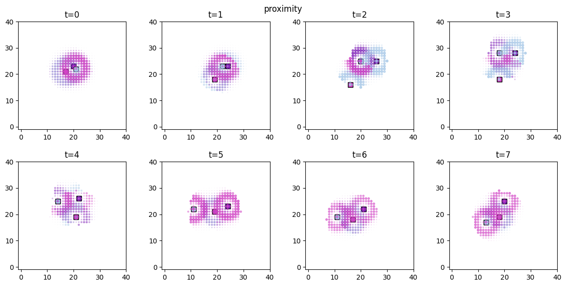
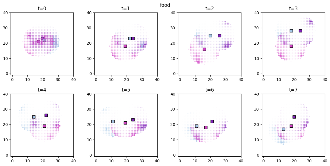
The spatial distributions of the values for each  and
and  can be conveniently visualized using
 plot_predictor helper function. The parameters are mostly self-explanatory. Note that predictors and scores are treated identically when passed to plot_predictor.
[14]:
for derived_quantity_name in random_foragers_sim.derived_quantities.keys():
ft.plot_predictor(
random_foragers_sim.foragers,
random_foragers_sim.derived_quantities[derived_quantity_name],
predictor_name=derived_quantity_name,
time=range(min(8, num_frames)),
grid_size=40,
size_multiplier=10,
random_state=99,
forager_position_indices=[0, 1, 2],
forager_predictor_indices=[0, 1, 2],
)
plt.suptitle(derived_quantity_name)
plt.show()
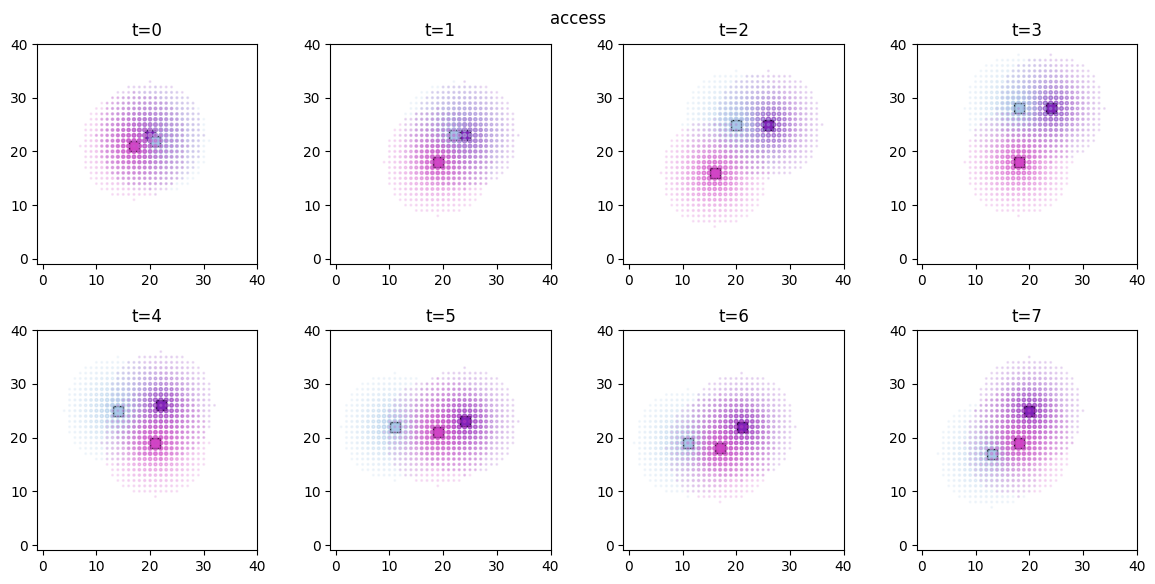
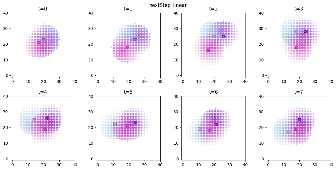
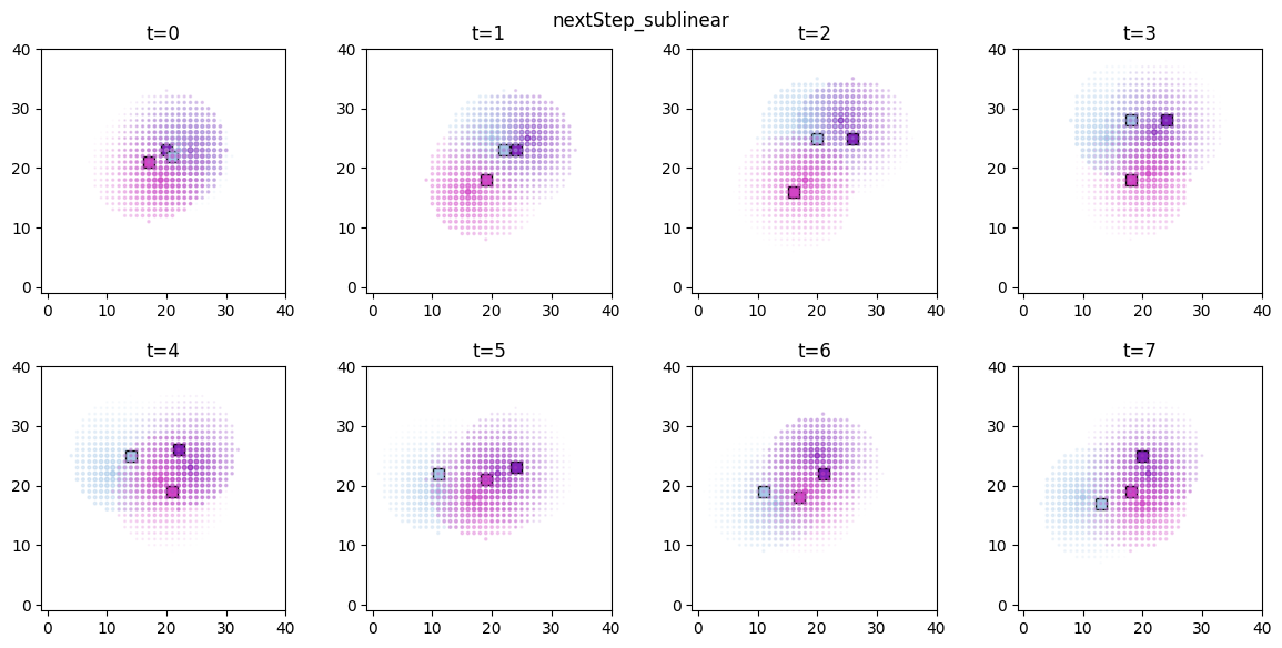
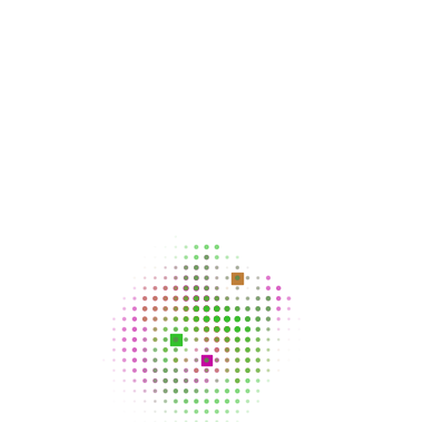
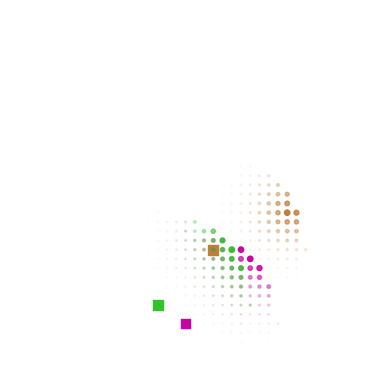
The time evolution of the derived values can be conveniently animated.
[15]:
ani = ft.animate_predictors(
random_foragers_sim.foragersDF,
random_foragers_sim.derived_quantities["proximity"],
predictor_name="proximity",
forager_position_indices=[0, 1, 2],
forager_predictor_indices=[0, 1, 2],
grid_size=40,
random_state=10,
size_multiplier=10,
)
HTML(ani.to_jshtml())
2024-10-28 13:54:33,739 - Animation.save using <class 'matplotlib.animation.HTMLWriter'>
50
[15]:
[16]:
ani = ft.animate_predictors(
random_foragers_sim.foragersDF,
random_foragers_sim.derived_quantities["food"],
predictor_name="food",
forager_position_indices=[0, 1, 2],
forager_predictor_indices=[0, 1, 2],
grid_size=40,
random_state=10,
size_multiplier=15,
)
HTML(ani.to_jshtml())
2024-10-28 13:54:35,987 - Animation.save using <class 'matplotlib.animation.HTMLWriter'>
50
[16]:
Inference
Now we fit the next step score as a linear combination of the predictors. We consider the following Bayesian model for the distribution of the score  :
:
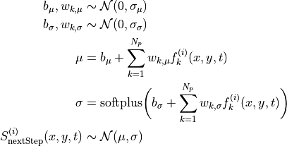
The priors for the latent variables are normal distributions centered at zero with standard deviations set to slightly regularizing values of 0.6, 0.2, that is,  and
and  , respectively. Recall that
  .
.
The inference task is: given the values of the actual (observed) score values  and the predictor values
  (these are precisely the derived quantities computed previously), find the posterior distributions of the
  parameters
  . For that goal we use the pyro package, a popular Python-based universal probabilistic
programming framework.
Our eventual parameters of interest are the  . Roughly speaking, this corresponds to the predictive relationship

We start by preparing the training data as tensor dictionaries. All the data is flattened to 1D.
[17]:
predictors = ["proximity_scaled", "food_scaled", "access_scaled"]
outcome_vars = ["nextStep_sublinear"]
predictor_tensors_random, outcome_tensor_random = ft.prep_data_for_inference(
random_foragers_sim, predictors, outcome_vars
)
predictor_tensors_random, outcome_tensor_random
2024-10-28 13:54:38,362 - Sample size: 43675
[17]:
({'proximity_scaled': tensor([0.5239, 0.5618, 0.5787, ..., 0.5725, 0.6671, 0.5055]),
'food_scaled': tensor([0.3077, 0.2762, 0.2844, ..., 0.5081, 0.7455, 0.1851]),
'access_scaled': tensor([0.0000, 0.0048, 0.0169, ..., 0.0169, 0.0048, 0.0000])},
{'nextStep_sublinear': tensor([0.0000, 0.0143, 0.0238, ..., 0.1496, 0.1343, 0.1088])})
[18]:
# plot outcome vs predictors
ft.visualise_forager_predictors(
predictors=[
predictor_tensors_random["proximity_scaled"],
predictor_tensors_random["food_scaled"],
predictor_tensors_random["access_scaled"],
],
predictor_names=["proximity_scaled", "food_scaled", "access_scaled"],
outcome_name="nextStep_sublinear",
outcome=outcome_tensor_random["nextStep_sublinear"],
sampling_rate=0.5,
)
Now we create the Pyro model.
[19]:
model_sigmavar_random = ft.HeteroskedasticLinear(
predictor_tensors_random, outcome_tensor_random
)
pyro.render_model(
model_sigmavar_random,
model_args=(predictor_tensors_random, outcome_tensor_random),
# render_deterministic=True, # this requires Pyro>1.9
)
[19]:
Aside for the two bias terms, for each predictor  we have 2 associated variables in the above (generalized) linear Gaussian model:
weightfor the mean ( above),
weightfor the standard deviation ( above).
The get_samples function runs the Stochastic Variational Inference algorithm in Pyro and returns a results dictionary with the following keys:
samples: the actual samples from the posterior predictive distribution. A dictionary indexed by the inferred variable names (see above),guide: thepyroguide object used in the SVI algorithm,predictive: an instance ofpyro.infer.Predictivecapable of generating new samples if need be.
[20]:
results_random = ft.get_samples(
model=model_sigmavar_random,
predictors=predictor_tensors_random,
outcome=outcome_tensor_random,
num_svi_iters=1500,
num_samples=1000,
)
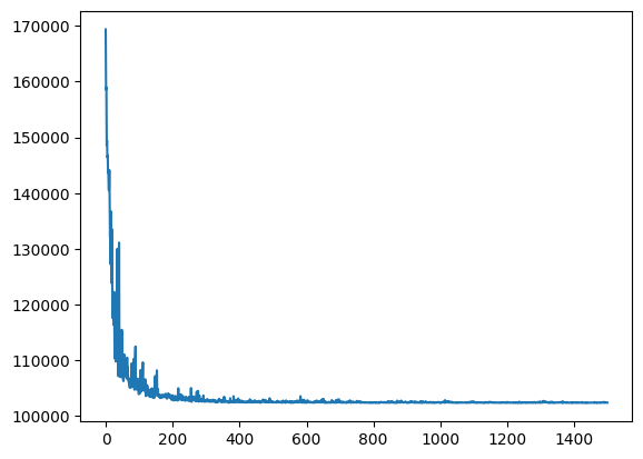
2024-10-28 13:54:39,323 - Starting SVI inference with 1500 iterations.
[iteration 0001] loss: 169343.6719
[iteration 0200] loss: 103110.3047
[iteration 0400] loss: 102820.6016
[iteration 0600] loss: 102484.0312
[iteration 0800] loss: 102495.9297
[iteration 1000] loss: 102464.2891
[iteration 1200] loss: 102411.2266
[iteration 1400] loss: 102442.7188
2024-10-28 13:54:49,412 - SVI inference completed in 10.09 seconds.
Coefficient marginals:
Site: weight_continuous_proximity_scaled_nextStep_sublinear
mean std 5% 25% 50% 75% 95%
0 0.024934 0.013398 0.00314 0.015859 0.025298 0.033872 0.047168
Site: weight_continuous_food_scaled_nextStep_sublinear
mean std 5% 25% 50% 75% 95%
0 -0.021922 0.0116 -0.040728 -0.029849 -0.022157 -0.014026 -0.003171
Site: weight_continuous_access_scaled_nextStep_sublinear
mean std 5% 25% 50% 75% 95%
0 0.64597 0.014731 0.620537 0.636394 0.646301 0.65577 0.669115
We can now visualize the posterior distributions of the parameters  .
.
[21]:
selected_sites = [
key
for key in results_random["samples"].keys()
if key.startswith("weight") and not key.endswith("sigma")
]
selected_samples = {key: results_random["samples"][key] for key in selected_sites}
ft.plot_coefs(
selected_samples, "Random foragers", nbins=120, ann_start_y=160, ann_break_y=50
)
# save the samples for future use if not present
if not os.path.exists("sim_data/random_foragers_samples.dill"):
with open(os.path.join("sim_data/random_foragers_samples.dill"), "wb") as f:
dill.dump(selected_samples, f)
As expected, the only nonzero coefficient is access. The access predictor is indeed independent from the other foragers or the food distribution, and depends solely on the distance between the forager and the target location.
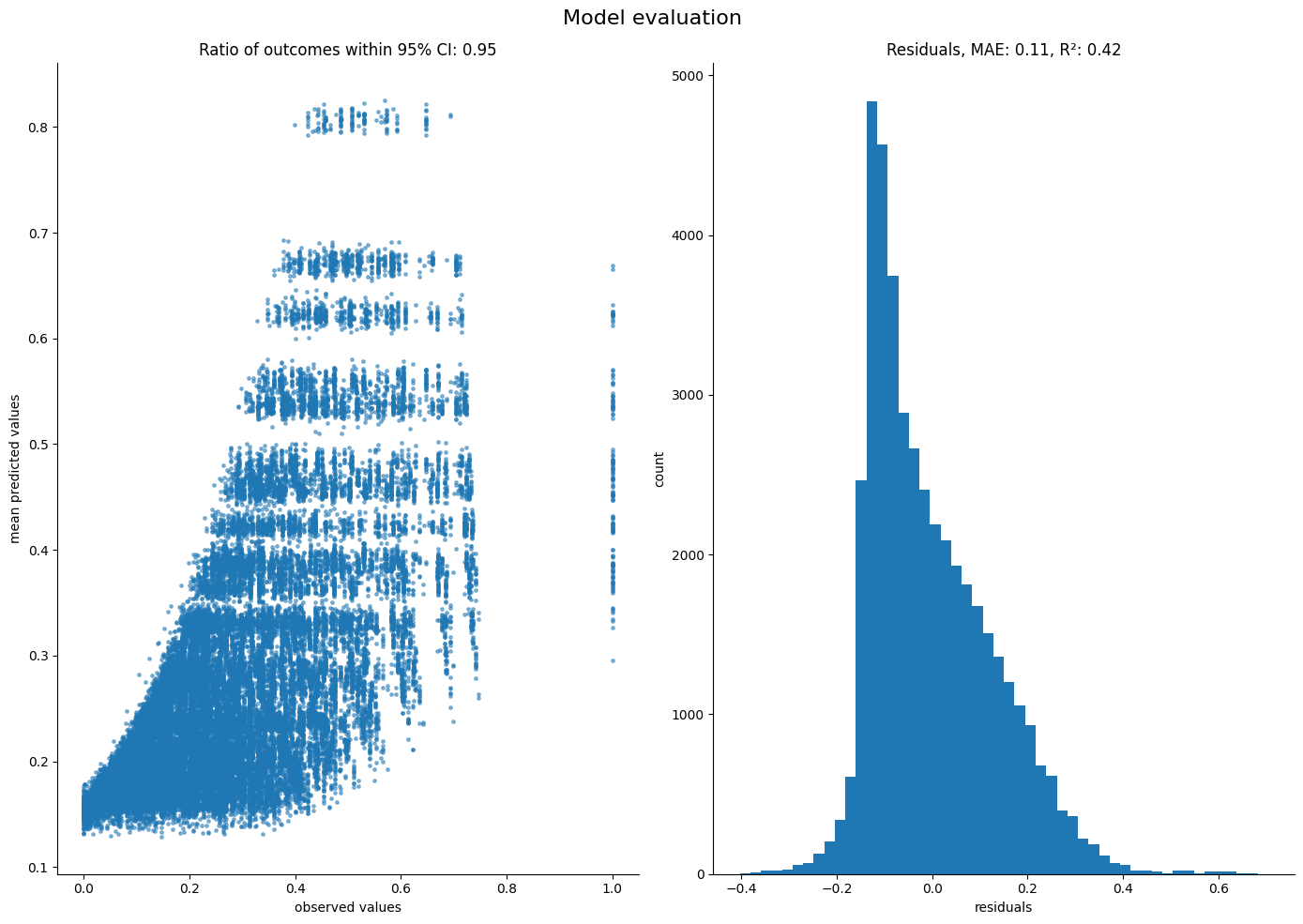
Finally we are able to compare the resulting predictive distribution with the observed data.
[22]:
ft.evaluate_performance(
model=model_sigmavar_random,
guide=results_random["guide"],
predictors=predictor_tensors_random,
outcome=outcome_tensor_random,
num_samples=1000,
)
