Foraging locust with dynamical systems (interpretation)

There are four notebooks on the dynamical systems analysis of the locust data, which should be read in the following order:

• locust_ds_data.ipynb

• locust_ds_class.ipynb

• locust_ds_validate.ipynb

• locust_ds_interpret.ipynb

In the notebook of this series, we briefly explain how the estimated parameters of the dynamical systems model are to be interpreted.

import os

import dill
import matplotlib.pyplot as plt
import pyro
import seaborn as sns

pyro.settings.set(module_local_params=True)

sns.set_style("white")

seed = 123
pyro.clear_param_store()
pyro.set_rng_seed(seed)

import matplotlib.pyplot as plt
import seaborn as sns

from collab.foraging import locust as lc
from collab.utils import find_repo_root

locds = lc.LocustDS(
    data_code="15EQ20191202",
    start=0,
    end=10,
)

locds.run_inference(
    "length",
    num_iterations=1500,
    num_samples=150,
    lr=0.001,  # force=True, save=True
)

Loading inference samples

Having run inference, we inspect the third “wondering” coefficient and the fourth “attraction” product coefficient. If this looks confusing, the notational conventions are discussed in locust_ds_class.ipynb. Just as a reminder, w_feed is the coefficient that captures those locusts that are searchers (neither moving around the edge, nor feeding) and move towards food (on the left or on the right) just by exploration:

w_searchers_lf = w_feed * X["search_l"]
w_searchers_rf = w_feed * X["search_r"]

dX["search_l"]  = ... - w_searchers_lf ...
dX["feed_l"] = ... + w_searchers_lf  ...

In contrast, a_feed is a product coefficient, used in more flux terms. It captures the attraction of edgers (left/right) towards the feeding units - these flux terms are used to move edgers towards the next available compartment between edgers and feeding, i.e. searchers.

a_edgers_lf = a_feed * X["edge_l"] * X["feed_l"]
a_edgers_rf = a_feed * X["edge_r"] * X["feed_r"]

dX["search_l"] = ... + a_edgers_lf  ....
dX["edge_l"] =  ... - - a_edgers_lf  ...

It also is assumed to capture the attraction of searchers to feeding units:

a_searchers_lf = a_feed * X["search_l"] * X["feed_l"]
a_searchers_rf = a_feed * X["search_r"] * X["feed_r"]

dx["search_l] = ... - a_searchers_lf  ...
dX["feed_l"] =  ...  + a_searchers_lf ...

locds.get_prior_samples(num_samples=150)
locds.plot_param_estimates(3, 4)

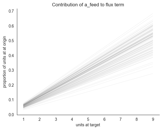
The key conceptual point here is that the w_-coefficients and the a-coefficients are not on the same scale. The former are ratios of origin compartments expected to depart at a time step, whereas to get an analogous ratio using an a_-coefficient, we need to first multiply it by the locust count at the target compartment. Here’s a visualization of how such a ratio depends on the target compartment counts for a realistic range of values (1-9).

lc.plot_ds_interaction(locds.samples, "attraction", 4, xlim=10, num_lines=100)

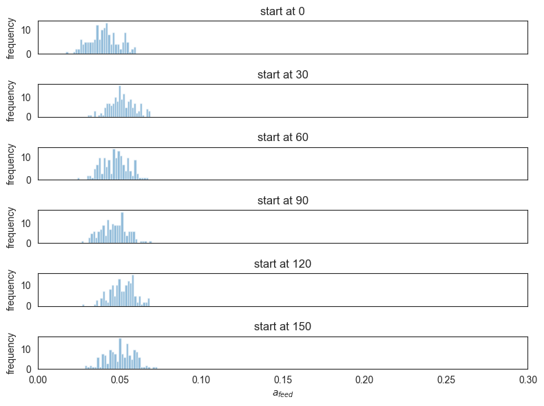
Another point we investigated was whether the estimated a_feed coefficient changes depending on the time window start, corresponding to the question of whether the locusts change their attraction to feeder throughout the experiment.

data_code = "15EQ20191202"

samples_a_feed_10 = []

root = find_repo_root()
data_path = os.path.join(root, f"data/foraging/locust/ds/locust_samples_a_feed_10.pkl")

if os.path.exists(data_path):
    with open(data_path, "rb") as f:
        samples_a_feed_10 = dill.load(f)
else:
    for start in [0, 30, 60, 90, 120, 150]:
        print(start)
        locds = lc.LocustDS(
            data_code=data_code,
            start=start,
            end=start + 10,
        )

        locds.run_inference("length", num_iterations=1500, num_samples=150, lr=0.001)
        samples_a_feed_10.append(locds.samples["attraction"][:, 4])

    with open(data_path, "wb") as f:
        dill.dump(samples_a_feed_10, f)

start = [0, 30, 60, 90, 120, 150]

fig, axs = plt.subplots(len(start), 1, figsize=(8, 6), sharex=True)

for i, (s, tensor) in enumerate(zip(start, samples_a_feed_10)):
    axs[i].hist(tensor, bins=30, alpha=0.5, label=f"start at {s}")
    axs[i].set_ylabel("frequency")
    axs[i].title.set_text(f"start at {s}")
    axs[i].set_xlim(0, 0.3)

axs[-1].set_xlabel("$a_{feed}$")
plt.tight_layout()
# plt.savefig("locust_a_feed_10_various_starts.png")
plt.show()