`Causal Explanations in Models with Continuous Random Variables <#toc0_>`__¶

The Explainable Reasoning with ChiRho module aims to provide a unified, principled approach to computations of causal explanations. We showed in an earlier tutorial how ChiRho provides SearchForExplanation, an effect handler that transforms causal probabilistic programs to compute causal explanations and other related causal queries. In that tutorial we focused on discrete variables. In this notebook, we illustrate the usage of SearchForExplanation for causal models with continuous random variables in the context of a dynamical system.

We take an epidemiological dynamical system model (described in more detail in our dynamical systems tutorial), expand it to a causal model with two interacting policies: lockdown and masking, where the former dampens the effect of the latter (the stronger the lockdown, the less the masking matters as people interact less anyway). Suppose both policies have been implemented, resulting in an undesirable overshoot (roughly, the ratio of people who infected after the peak of the epidemic). Given this outcome, we want to be able to isolate the relative causal role of lockdown and masking policies. In particular, we show how using ChiRho’s SearchForExplanation and Pyro’s probabilistic inference reflect the intuition that since lockdown dampened the masking effect, it was lockdown that caused the overshoot being too high, even if masking alone without lockdown would also have led to a similar consequence.

`Outline <#toc0_>`__¶

Setup
Bayesian Epidemiological SIR Model with Policies
But for Analysis with Bayesian SIR Model with Policies
Causal Explanations using SearchForExplanation
Fine-grained Analysis of overshoot using Sample traces
Looking into Different Contexts for Curious Readers
Conclusions

`Setup <#toc0_>`__¶

The main dependencies for this example are PyTorch, Pyro, and ChiRho.

[1]:

import numbers
import os
from typing import Tuple, TypeVar, Union, Optional, Callable
import math

import matplotlib.pyplot as plt
import pandas as pd
import pyro.distributions as dist
from pyro.distributions import constraints
import seaborn as sns
import torch
from pyro.infer import Predictive

import pyro
from chirho.counterfactual.handlers.counterfactual import MultiWorldCounterfactual
from chirho.dynamical.handlers.interruption import StaticEvent
from chirho.dynamical.handlers.solver import TorchDiffEq
from chirho.dynamical.handlers.trajectory import LogTrajectory
from chirho.dynamical.ops import Dynamics, State, on, simulate
from chirho.explainable.handlers import SearchForExplanation
from chirho.explainable.handlers.components import ExtractSupports
from chirho.indexed.ops import IndexSet, gather
from chirho.interventional.ops import Intervention, intervene
from chirho.observational.handlers import condition

R = Union[numbers.Real, torch.Tensor]
S = TypeVar("S")
T = TypeVar("T")


sns.set_style("white")

seed = 123
pyro.clear_param_store()
pyro.set_rng_seed(seed)

smoke_test = "CI" in os.environ
num_samples = 10 if smoke_test else 10000

`Bayesian Epidemiological SIR model with Policies <#toc0_>`__¶

We start with building the epidemiological SIR (Susceptible, Infected, Recovered) model, one step at a time. We first encode the deterministic SIR dynamics. Then we add uncertainty about the parameters that govern these dynamics: \(\beta\) and \(\gamma\). These parameters have been described in detail in the dynamical systems tutorial. We then incorporate the resulting model into a more complex causal model that involves two policy mechanisms: imposing lockdown and masking restrictions.

Our outcome of interest is overshoot, the proportion of the population that remains susceptible after the epidemic peaks but eventually becomes infected as the epidemic continues. One way to compute it is to:

Find the time when the number of infected individuals is at its peak, which we denote t_max.
Determine the proportion of susceptible individuals at t_max in the whole population, which we denote S_peak.
Find the proportion of susceptible individuals (and have thus never been infected) at the end of the logging period, S_final.
Return the difference between proportions of peak and final susceptible individuals, S_peak - S_final.

Epidemic mitigation policies often have multiple goals that must be balanced. One typical goal is to increase S_final, i.e., to limit the total number of infected individuals. Another goal is to limit the number of infected individuals at the peak of the epidemic to avoid overwhelming the healthcare system. Yet another goal is to minimize the proportion of the population that becomes infected after the peak, that is, the overshoot, to reduce healthcare and economic burdens. Balancing these objectives involves making trade-offs. To properly think through such trade-offs, one needs a decent counterfactual picture of what these outcomes might be under various interventions. In what follows, we focus on overshoot.

Suppose we are working under the constraint that the overshoot should be lower than 24% of the population, and we implement two public health policies, lockdown and masking, which together seem to lead to the overshoot being too high. As an example, we will work with an example when only one of them holds most of the responsibility, and we are interested in being able to identify which one.

`Assumptions <#toc0_>`__¶

We make a range of assumptions in this tutorial:

All dynamics in the system are deterministic, meaning that the system’s behavior can be precisely described by its current state and the governing equations without random variability, and all the stochasticity is delegated to parameter uncertainty and perhaps observational noise.
The dynamical system model is known except for the prameters, and accurately captures the process we want to model.
There are no confounders between the model parameters, i.e. these are not systematically influenced by unobserved variables in a way that would bias our causal effect estimates.

There are many models where we could relax or abandon these assumptions, which would lead to other modeling decisions. The general point, however, of how to use a model with SearchForCauses would, mutatis mutandis, hold as soon as one has a causal model.

`SIR Model and Simulation <#toc0_>`__¶

[2]:

# dS = - beta . SI
# dI = beta * SI - gamma * I
# dR = gamma * I

class SIRDynamics(pyro.nn.PyroModule):
    def __init__(self, beta, gamma):
        super().__init__()
        self.beta = beta
        self.gamma = gamma

    def forward(self, X: State[torch.Tensor]):
        dX: State[torch.Tensor] = dict()
        dX["S"] = -self.beta * X["S"] * X["I"]
        dX["I"] = self.beta * X["S"] * X["I"] - self.gamma * X["I"]
        dX["R"] = self.gamma * X["I"]

        return dX


# l is a parameter describing the strength of the intervening policies
# it is a value between 0 and 1, and (1-l) is the fraction of the original unintervened beta
class SIRDynamicsPolicies(SIRDynamics):
    def __init__(self, beta0, gamma):
        super().__init__(beta0, gamma)
        self.beta0 = beta0

    def forward(self, X: State[torch.Tensor]):
        self.beta = (1 - X["l"]) * self.beta0
        dX = super().forward(X)
        dX["l"] = torch.zeros_like(X["l"])
        return dX

[3]:

# Computing overshoot in a simple SIR model without interventions
# note it's below the desired threshold

total_population = 100
init_state = dict(S=torch.tensor(99.0), I=torch.tensor(1.0), R=torch.tensor(0.0))
assert init_state["S"] + init_state["I"] + init_state["R"] == total_population

start_time = torch.tensor(0.0)
end_time = torch.tensor(12.0)
step_size = torch.tensor(0.1)
logging_times = torch.arange(start_time, end_time, step_size)
init_state_lockdown = dict(**init_state, l=torch.tensor(0.0))

# We now simulate from the SIR model
beta_true = torch.tensor([0.03])
gamma_true = torch.tensor([0.5])
sir_true = SIRDynamics(beta_true, gamma_true)
with TorchDiffEq(), LogTrajectory(logging_times) as lt:
    simulate(sir_true, init_state, start_time, end_time)

sir_true_traj = lt.trajectory


def get_overshoot(trajectory):
    t_max = torch.argmax(trajectory["I"].squeeze())
    S_peak = torch.max(trajectory["S"].squeeze()[t_max]) / total_population
    S_final = trajectory["S"].squeeze()[-1] / total_population
    return (S_peak - S_final).item()


print(get_overshoot(sir_true_traj))

0.15116800367832184

The number \(0.15\) is the overshoot you get if \(\beta = 0.03, \gamma = 0.5\), which, say, are the true parameters of the epidemic. This value is observed by simulating the SIR dynamics model with these values and calculating the overshoot directly.

Also, note that the above dynamical system introduces the variables: S - susceptible, I - infected, R - recovered, and l - effect of the intervention. These variables evolve over time and their dynamics are captured by the model. As we add features to our model, we also add new variables to this list. Further on in the notebook, we will describe the probabilities we compute in terms of these variables.

`Bayesian SIR model <#toc0_>`__¶

Now suppose we are uncertain about \(\beta\) and \(\gamma\), and want to construct a Bayesian SIR model that incorporates this uncertainty. Say we induce \(\beta\) to be drawn from the distribution Beta(18, 600), and \(\gamma\) to be drawn from distribution Beta(1600, 1600). This converts the parameters of the original dynamical system into random variables beta and gamma in our model.

[4]:

# Defining a Bayesian SIR model where we have priors over beta and gamma distributions

def bayesian_sir(base_model=SIRDynamics) -> Dynamics[torch.Tensor]:
    beta = pyro.sample("beta", dist.Beta(18, 600))
    gamma = pyro.sample("gamma", dist.Beta(1600, 1600))
    sir = base_model(beta, gamma)
    return sir


def simulated_bayesian_sir(
    init_state, start_time, logging_times, base_model=SIRDynamics
) -> State[torch.Tensor]:
    sir = bayesian_sir(base_model)

    with TorchDiffEq(), LogTrajectory(logging_times, is_traced=True) as lt:
        simulate(sir, init_state, start_time, logging_times[-1])
    return lt.trajectory

`Bayesian SIR model with Policies <#toc0_>`__¶

Now we incorporate the Bayesian SIR model into a larger model that includes the effect of two different policies, lockdown and masking, where each can be implemented with \(50\%\) probability. These probabilities won’t really matter, as we will be intervening on these, the sampling is mainly used to register the parameters with Pyro. It does, hower, illustrate that the model in principle could incorporate uncertainties of this sort. We encode the intervention efficiencies which further affect the model. Crucially, these efficiencies interact in a fashion resembling the structure of the stone-throwing example we discussed in the tutorial on categorical variables. If a lockdown is present, this limits the impact of masking as agents interact less and so masks have fewer opportunities to block anything. We assume the situation is asymmetric: masking has no impact on the efficiency of lockdown. The model also computes overshoot and os_too_high for further analysis.

[5]:

# a utility function
# allowing for interventions on a dynamical system
# within another model
# to avoid conflicts arising from repeated sites in the trace

def MaskedStaticIntervention(time: R, intervention: Intervention[State[T]]):

    @on(StaticEvent(time))
    def callback(
        dynamics: Dynamics[T], state: State[T]
    ) -> Tuple[Dynamics[T], State[T]]:

        with pyro.poutine.block():
            return dynamics, intervene(state, intervention)

    return callback

[6]:

# Defining the policy model

overshoot_threshold = 24
lockdown_time = torch.tensor(1.0)
mask_time = torch.tensor(1.5)

def policy_model() -> State[torch.Tensor]:

    lockdown = pyro.sample("lockdown", dist.Bernoulli(torch.tensor(0.5)))
    mask = pyro.sample("mask", dist.Bernoulli(torch.tensor(0.5)))

    lockdown_efficiency = pyro.deterministic(
        "lockdown_efficiency", torch.tensor(0.6) * lockdown, event_dim=0
    )

    mask_efficiency = pyro.deterministic(
        "mask_efficiency", (0.1 * lockdown + 0.45 * (1 - lockdown)) * mask, event_dim=0
    )

    joint_efficiency = pyro.deterministic(
        "joint_efficiency",
        torch.clamp(lockdown_efficiency + mask_efficiency, 0, 0.95),
        event_dim=0,
    )

    lockdown_sir = bayesian_sir(SIRDynamicsPolicies)
    with LogTrajectory(logging_times, is_traced=True) as lt:
        with TorchDiffEq():
            with MaskedStaticIntervention(lockdown_time, dict(l=lockdown_efficiency)):
                with MaskedStaticIntervention(mask_time, dict(l=joint_efficiency)):
                    simulate(
                        lockdown_sir, init_state_lockdown, start_time, logging_times[-1]
                    )

    return lt.trajectory

def overshoot_query(trajectory: State[torch.Tensor]) -> Tuple[torch.Tensor, torch.Tensor]:

    t_max = torch.max(trajectory["I"], dim=-1).indices
    S_peaks = pyro.ops.indexing.Vindex(trajectory["S"])[..., t_max]
    overshoot = pyro.deterministic(
        "overshoot", S_peaks - trajectory["S"][..., -1], event_dim=0
    )
    os_too_high = pyro.deterministic(
        "os_too_high",
        (overshoot > overshoot_threshold).clone().detach().float(),
        event_dim=0,
    )

    return overshoot, os_too_high

def overshoot_model():
    trajectory = policy_model()
    return overshoot_query(trajectory)

Now that we have our full-fledged model of SIR dynamics along with interventions, we have a complete list of random variables in question. In our explanations, we will abbreviate them as follows.

S - susceptible,
I - infected,
R - recovered,
l - the effect of intervention,
beta, gamma - the parameters of the SIR dynamics model,
ld - lockdown,
m - masking,
le - lockdown efficiency,
me - mask efficiency,
je - joint efficiency,
os - overshoot, and
oth - overshoot is too high.

We use these notations in the rest of the notebook to describe the probabilities we are computing.

`But-for Analysis with Bayesian SIR model with Policies <#toc0_>`__¶

Suppose now we introduced both policies and overshoot in fact was too high. As a first attempt at explaining why this happened, we may begin with an analysis of but-for causation. Recall from our previous tutorial, that the key idea behind but-for analysis is to evaluate whether “\(B\) wouldn’t have been the case but for \(A\) happening”. In this case, we want to know whether the overshoot still would have been too high had we not imposed a lockdown and/or a masking policy.

To apply but-for analysis in this case, we investigate the following four scenarios:

None of the policies were applied
Both lockdown and masking were enforced
Only masking was imposed
Only lockdown was imposed

We create four models representing each of these scenarios by conditioning our original overshoot_model on the variables representing whether each policy was applied, lockdown and mask. For the sake of completeness, we also illustrate the consequences of following a stochastic policy and deciding randomly about the interventions.

[7]:

# conditioning (as opposed to intervening) is sufficient for
# propagating the changes, as the decisions are upstream from ds

# no interventions
overshoot_model_none = condition(
    overshoot_model, {"lockdown": torch.tensor(0.0), "mask": torch.tensor(0.0)}
)
unintervened_predictive = Predictive(
    overshoot_model_none, num_samples=num_samples, parallel=True
)
unintervened_samples = unintervened_predictive()

# both interventions
overshoot_model_all = condition(
    overshoot_model, {"lockdown": torch.tensor(1.0), "mask": torch.tensor(1.0)}
)
intervened_predictive = Predictive(
    overshoot_model_all, num_samples=num_samples, parallel=True
)
intervened_samples = intervened_predictive()

overshoot_model_mask = condition(
    overshoot_model, {"lockdown": torch.tensor(0.0), "mask": torch.tensor(1.0)}
)
mask_predictive = Predictive(overshoot_model_mask, num_samples=num_samples, parallel=True)
mask_samples = mask_predictive()

overshoot_model_lockdown = condition(
    overshoot_model, {"lockdown": torch.tensor(1.0), "mask": torch.tensor(0.0)}
)
lockdown_predictive = Predictive(
    overshoot_model_lockdown, num_samples=num_samples, parallel=True
)
lockdown_samples = lockdown_predictive()

predictive = Predictive(overshoot_model, num_samples=num_samples, parallel=True)
samples = predictive()

print("Variables in the model:", samples.keys())

Variables in the model: dict_keys(['lockdown', 'mask', 'beta', 'gamma', 'lockdown_efficiency', 'mask_efficiency', 'joint_efficiency', 'S', 'I', 'R', 'l', 'overshoot', 'os_too_high'])

Note that the above list of variables matches our list of variables earlier when we constructed the full-fledged SIR model.

[8]:

def add_pred_to_plot(preds, axs, coords, color, label):
    sns.lineplot(
        x=logging_times,
        y=preds.mean(dim=0).squeeze().tolist(),
        ax=axs[coords],
        label=label,
        color=color,
    )
    axs[coords].fill_between(
        logging_times,
        torch.quantile(preds, 0.025, dim=0).squeeze(),
        torch.quantile(preds, 0.975, dim=0).squeeze(),
        alpha=0.2,
        color=color,
    )


fig, axs = plt.subplots(5, 2, figsize=(12, 7.5))

colors = ["orange", "red", "green"]

add_pred_to_plot(
    unintervened_samples["S"], axs, coords=(0, 0), color=colors[0], label="susceptible"
)
add_pred_to_plot(
    unintervened_samples["I"], axs, coords=(0, 0), color=colors[1], label="infected"
)
add_pred_to_plot(
    unintervened_samples["R"], axs, coords=(0, 0), color=colors[2], label="recovered"
)

axs[0, 0].set_title("No interventions")
for ax in axs[:, 0]:
    ax.set_xlabel("time")
    ax.set_ylabel("count")


for ax in axs[:, 1]:
    ax.set_xlim(0, 35)
    ax.set_xlabel("overshoot")
    ax.set_ylabel("num samples")

axs[0, 1].hist(unintervened_samples["overshoot"].squeeze())


axs[0, 1].set_title(
    f"Overshoot mean (no interventions): {unintervened_samples['overshoot'].squeeze().mean().item():.2f}, Pr(too high): {unintervened_samples['os_too_high'].squeeze().float().mean().item():.2f} "
)
axs[0, 1].axvline(unintervened_samples['overshoot'].squeeze().mean().item(), color="red",
                  linestyle="--", label="mean overshoot")
axs[0, 1].axvline(overshoot_threshold, color="black", linestyle="--", label="overshoot threshold")
axs[0, 1].legend()

add_pred_to_plot(
    intervened_samples["S"], axs, coords=(1, 0), color=colors[0], label="susceptible"
)
add_pred_to_plot(
    intervened_samples["I"], axs, coords=(1, 0), color=colors[1], label="infected"
)
add_pred_to_plot(
    intervened_samples["R"], axs, coords=(1, 0), color=colors[2], label="recovered"
)
axs[1, 0].set_title("Both interventions")
axs[1, 0].legend_.remove()


axs[1, 1].hist(intervened_samples["overshoot"].squeeze())
axs[1, 1].set_title(
    f"Overshoot mean (both interventions): {intervened_samples['overshoot'].squeeze().mean().item():.2f}, Pr(too high): {intervened_samples['os_too_high'].squeeze().float().mean().item():.2f} "
)
axs[1,1].axvline(intervened_samples['overshoot'].squeeze().mean().item(), color="red",
                linestyle="--", label="mean overshoot")
axs[1, 1].axvline(overshoot_threshold, color="black", linestyle="--", label="overshoot threshold")


add_pred_to_plot(
    mask_samples["S"], axs, coords=(2, 0), color=colors[0], label="susceptible"
)
add_pred_to_plot(
    mask_samples["I"], axs, coords=(2, 0), color=colors[1], label="infected"
)
add_pred_to_plot(
    mask_samples["R"], axs, coords=(2, 0), color=colors[2], label="recovered"
)
axs[2, 0].set_title("Mask only")
axs[2, 0].legend_.remove()

axs[2, 1].hist(mask_samples["overshoot"].squeeze())
axs[2, 1].set_title(
    f"Overshoot mean (mask only): {mask_samples['overshoot'].squeeze().mean().item():.2f}, Pr(too high): {mask_samples['os_too_high'].squeeze().float().mean().item():.2f} "
)
axs[2, 1].axvline(mask_samples['overshoot'].squeeze().mean().item(), color="red",
                linestyle="--", label="mean overshoot")
axs[2, 1].axvline(overshoot_threshold, color="black", linestyle="--", label="overshoot threshold")

add_pred_to_plot(
    lockdown_samples["S"], axs, coords=(3, 0), color=colors[0], label="susceptible"
)
add_pred_to_plot(
    lockdown_samples["I"], axs, coords=(3, 0), color=colors[1], label="infected"
)
add_pred_to_plot(
    lockdown_samples["R"], axs, coords=(3, 0), color=colors[2], label="recovered"
)
axs[3, 0].set_title("Lockdown only")
axs[3, 0].legend_.remove()

axs[3, 1].hist(lockdown_samples["overshoot"].squeeze())
axs[3, 1].set_title(
    f"Overshoot mean (lockdown only): {lockdown_samples['overshoot'].squeeze().mean().item():.2f}, Pr(too high): {lockdown_samples['os_too_high'].squeeze().float().mean().item():.2f} "
)
axs[3, 1].axvline(lockdown_samples['overshoot'].squeeze().mean().item(), color="red",
                linestyle="--", label="mean overshoot")
axs[3, 1].axvline(overshoot_threshold, color="black", linestyle="--", label="overshoot threshold")

add_pred_to_plot(samples["S"], axs, coords=(4, 0), color=colors[0], label="susceptible")
add_pred_to_plot(samples["I"], axs, coords=(4, 0), color=colors[1], label="infected")
add_pred_to_plot(samples["R"], axs, coords=(4, 0), color=colors[2], label="recovered")
axs[4, 0].set_title("Stochastic interventions with equal probabilities")
axs[4, 0].legend_.remove()

axs[4, 1].hist(samples["overshoot"].squeeze())
axs[4, 1].set_title(
    f"Overshoot mean (stochastic interventions): {samples['overshoot'].squeeze().mean().item():.2f}, Pr(too high): {samples['os_too_high'].squeeze().float().mean().item():.2f} "
)
axs[4, 1].axvline(samples['overshoot'].squeeze().mean().item(), color="red",
                linestyle="--", label="mean overshoot")
axs[4, 1].axvline(overshoot_threshold, color="black", linestyle="--", label="overshoot threshold")


fig.tight_layout()
fig.suptitle(
    "Trajectories and overshoot distributions in the but-for analysis",
    fontsize=16,
    y=1.05,
)
sns.despine()

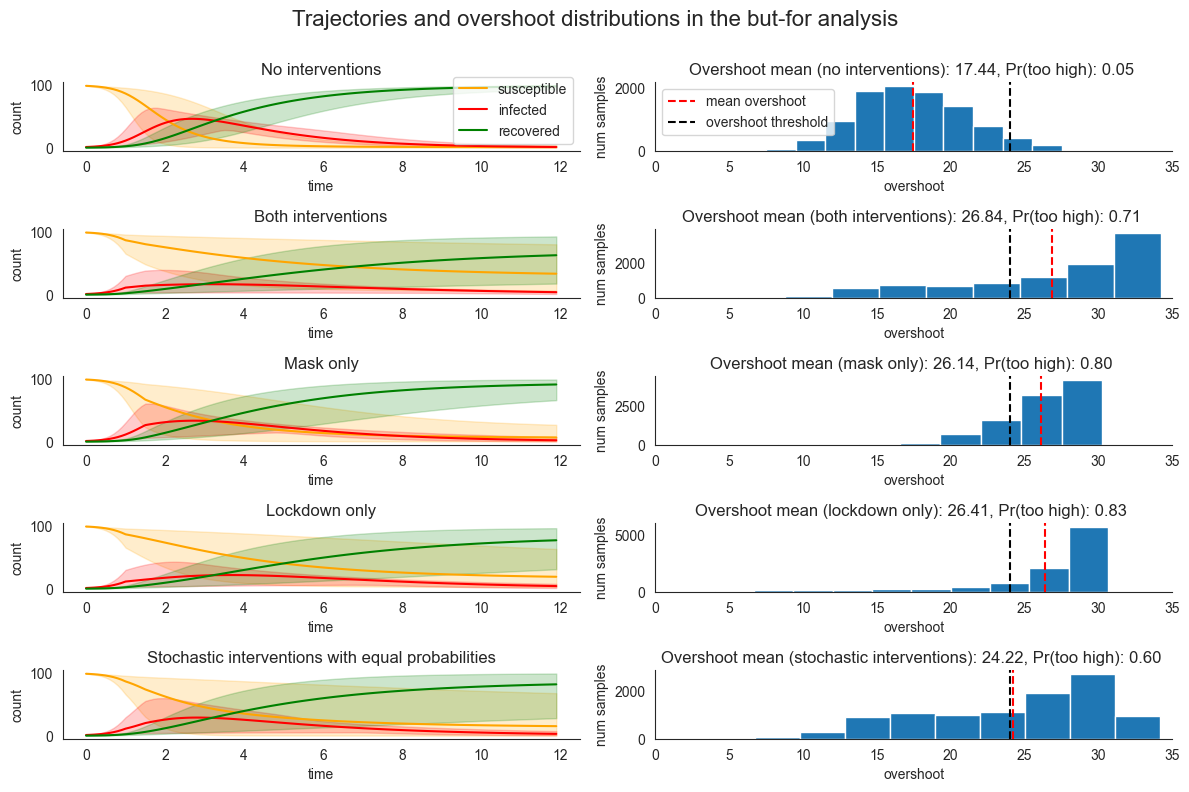
The plots above show what happens in each of the different scenarios. We observe that in the model where none of the policies were imposed, the probability of the overshoot being too high is relatively low, \(\approx 0.05\). On the other hand, when both policies were imposed, the probability of the overshoot being too high was relatively high at \(\approx 0.7\). In other words, the lockdown would not have happened if either or both of the policies had not been imposed.

To identify whether lockdown or mask is a singular cause under our but-for analysis, we compare the overshoot probability in the remaining models where only one intervention was applied. Interestingly, the effect of each intervention is somewhat nuanced. While implementing both interventions increases the risk of overshooting as compared to the no-intervention model, the probability of an overshoot is actually higher when either of the policies are imposed in isolation.

This simple but-for analysis fails to capture more fine-grained insights about how lockdown and mask influence the presence of an overshoot. To further refine our analysis we can use ChiRho’s SearchForExplanation capabilities, which accounts for the contribution of various potential causes in a range of possible context. As we showed in our previous tutorial, we achieve a greater level of sensitivity by stochastically keeping other variables in the model fixed at their original values. As we’ll see in the next section, there is a collections of variables such that if we keep them fixed, removing the lockdown would significantly lower the overshoot, but there is no context that we could keep fixed such that if we remove the masking policy, the overshoot would decrease. In the next section, we show how this analysis can be carried out with the help of SearchForExplanation.

`Causal Explanations using SearchForExplanation <#toc0_>`__¶

Before we dive into the code below, let us first define some notation. We use lower case abbreviations to refer to the value of the variables under consideration. For example, \(\mathit{ld}\) refers to lockdown=1 and \(\mathit{ld\,}'\) refers to lockdown=0. We place interventions in the subscripts, for instance, \(\mathit{os}_{\mathit{ld}}\) refers to the overshoot under the intervention that lockdown=1. Later on in the notebook, we also employ contexts that are kept fixed in the intervened worlds. We place these contexts in the superscript. For example, \(\mathit{os}_{\mathit{ld}}^{\mathit{me}}\) refers to the variable overshoot when lockdown was intervened to be 1 and mask_efficiency was kept fixed at its factual value.

We use \(P(.)\) to denote the distribution described by the model (overshoot_model in this notebook). We also induce a distribution over the sets of potential interventions and the sets of context nodes potentially kept fixed. We denote these distributions by \(P_a(.)\) and \(P_w(.)\) respectively. As an example, \(P_a(\{ld\})\) refers to the probability that the set of interventions under consideration is \(\{ld\}\). These distributions are determined using the parameters antecedent_bias and witness_bias given to the handler SearchForExplanation. For more details, please refer to the documentation.

At a high level, we will transform the original model into one that runs through three “possible worlds” at the same time.

The “actual world”, where the model is executed in its original unintervened form,
the “necessity world”, where the model is executed with changes to antecedents, and
the “sufficiency world”, where we fix the causal candidates at their actual values.

Then, using this collection of transformed models we’ll search over causal candidates, preferring those that can yield different outcomes in the “necessity world” and those that can yield similar outcomes in the “sufficiency world”. This search procedure will involve multiple runs which contain different interventional settings on multiple subsets of causal nodes and witnesses, and supported by Pyro’s automated machinery for probabilsitic inference. For a more detailed explanation of how this works, see our tutorial on explanation with categorical variables.

Now let’s dive into the code, using this notation to describe the quantities we are computing.

We first introduce a function for performing importance sampling through the model that returns cumulative log probabilities of the samples, sample traces, an effect handler object for multi-world counterfactual reasoning, and log probabilities. We use these objects later in the code to subselect the samples.

[9]:

def importance_infer(model: Optional[Callable] = None, *, num_samples: int):

    if model is None:
        return lambda m: importance_infer(m, num_samples=num_samples)

    def _wrapped_model(*args, **kwargs):

        guide = pyro.poutine.block(hide_fn=lambda msg: msg["is_observed"])(model)

        max_plate_nesting = 9  # TODO guess

        with pyro.poutine.block(), MultiWorldCounterfactual() as mwc_imp:
            log_weights, importance_tr, _ = (
                pyro.infer.importance.vectorized_importance_weights(
                    model,
                    guide,
                    *args,
                    num_samples=num_samples,
                    max_plate_nesting=max_plate_nesting,
                    normalized=False,
                    **kwargs
                )
            )

        return (
            torch.logsumexp(log_weights, dim=0) - math.log(num_samples),
            importance_tr,
            mwc_imp,
            log_weights,
        )

    return _wrapped_model

The key idea here is that once we transform the original model using SearchForExplanation the trace will not only contain the original sites, but also sites representing witness preemptions, sites representing which antecedents were intervened on, and sites representing differences between the values of the outcome variable across counterfactual worlds. At a high level, we’d be using a trace with the following structure:

A	Witness A	Antecedent A	B	Witness B	Antecedent B	…	Outcome	Outcome Diff
…	…	…	…	…	…	…	…	…

where each of these is tracked in each of the three transformed worlds described above (actual, necessity, and sufficiency). This collection of values will come with a corresponding “table” of importance weights for each sample, which will be the sum of the log probabilities wherever values are sampled from a distribution, and an additional set of terms for soft equality or soft non-equality on the outcome in “necessity” and “sufficiency” worlds. This way, we can exploit the already existing inference method to obtain samples and importance weights that capture answers to counterfactual queries.

Note: The particular choice of inference method used here is entirely interchangable with other inference methods supported by Pyro. The more important point is that SearchForExplanation recasts search into standard probabilistic inference.

Then, we set up the query as follows:

supports: We extract the support of each distribution in the model using ExtractSupports. We also encode our knowledge that os_too_high is a Boolean. Note that constraints for deterministic nodes currently need to be specified manually when using ExtractSupports, as we do here.
antecedents: We postulate lockdown=1 and mask=1 as possible causes.
alternatives: We provide lockdown=0 and mask=0 as alternative values. If we don’t specify them, the search simply samples the values using uniform/wide distributions for those sites - which makes sense if the site has continuous support or if we only know the outcome but not the antecedent values. For this simpler application, however, searching through lockdown=1 or mask=1 as alternatives would not conceptually do, as we already know what the alternative values should be.
witnesses: We includemask_efficiencyandlockdown_efficiency` as candidates to be included in the contexts potentially to be kept fixed.
consequents: We put os_too_high=1 as the outcome whose causes we wish to analyze.
antecedent_bias, witness_bias: We set these parameters to have equal probabilities of intervening on cause candidates, and to slightly prefer smaller witness sets. Please refer to the documentation of SearchForExplanation for more details.
consequent_scale is set to effectively lead to probabilities near 0 and 1 depending on whether the binary outcomes differ across counterfactual worlds.

[10]:

with ExtractSupports() as s:
    overshoot_model()

supports = s.supports
supports["os_too_high"] = constraints.independent(
    base_constraint=constraints.boolean, reinterpreted_batch_ndims=0
)

query = SearchForExplanation(
    supports=supports,
    alternatives={"lockdown": torch.tensor(0.0), "mask": torch.tensor(0.0)},
    antecedents={"lockdown": torch.tensor(1.0), "mask": torch.tensor(1.0)},
    antecedent_bias=0.0,
    witnesses={
        key: s.supports[key] for key in ["lockdown_efficiency", "mask_efficiency"]
    },
    consequents={"os_too_high": torch.tensor(1.0)},
    consequent_scale=1e-8,
    witness_bias=0.2,
)(overshoot_model)

logp, importance_tr, mwc_imp, log_weights = importance_infer(num_samples=num_samples)(query)()
print(torch.exp(logp))

tensor(0.1328)

The SearchForExplanation effect handler constructs a probabilistic model representing two stochastic searches at the same time; which antecedants to intervene on, and which witnesses to keep fixed at their original values. These search procedures are represented as random choices in the constructed query Pyro program. Executions of this model capture random choices within the model itself, as well as random choices representing one configuration of the search procedure. For this reason, log probabilities under the query model are impacted by both uncertainties present in the original model and the probabilistic search distributions. But also, this means there is some nuance as to how to interpret and how to decompose them. Let’s talk this through.

The above probability itself, which potentially is of interest in some applications when one-number summaries are a good enough approximation, is only related to our current query. It is the probability that the overshoot is both too high in the antecedents-intervened world and not too high in the alternatives-intervened world, where antecedent interventions are preempted with probabilities \(0.5\) at each site, and witnesses are kept fixed at the observed values with probability \(0.5+0.2\) at each site (see the tutorial on categorical variables for an explanation of why this stochasticity is in general useful). Given how search and model stochasticities are composed here, we expect these values to not be very high - but them being so does not mean low causal role.

Now, more fine-grained queries can be answered using the 10000 samples we have drawn in the process. We first compute the probabilities that different sets of antecedent candidates have a causal effect over os_too_high conditioned on the fact that lockdown and masking were actually imposed in the factual world. This conditioning grounds out our explanations in terms of what actually happened in the particular instance we are interested in.

Note: There are many alternative definitions for actual causation or explanation that can make use of the same query program, only changing how the log probabilities are interpretted. For example, one may prefer smaller causal sets, or they may prefer higher context sensitivity, both of which can be tuned and are mirrored in the resulting log probabilities.

[11]:

def compute_prob(trace, log_weights, mask, verbose=True):
    mask_intervened = torch.ones(
        trace.nodes["__cause____antecedent_lockdown"]["value"].shape
    ).bool()
    for i, v in mask.items():
        mask_intervened &= trace.nodes[i]["value"] == v

    prob = (torch.sum(torch.exp(log_weights) * mask_intervened.squeeze()) / mask_intervened.float().sum()).item()

    if verbose:
        print(mask, prob)

    return prob

We specifically compute the following four probabilities. In each of the computations, we condition on lockdown and masking actually being implemented in the factual world. Given this factual world, each equation represents the probability that a given collection of policy interventions would have changed whether the overshoot was too high. For instance, in equation 1., we assume lockdown (ld) and masking (m) have been implemented, and we ask about the joint probability that both (a) removing both interventions, i.e. intervening for both ld and m to not happen - which we mark by the apostrophe - would lead to oth not happening, \(\mathit{oth}'_{\mathit{ld'}, m'}\), and (b) intervening for both to happen would lead to oth, \(\mathit{oth}_{\mathit{ld}, m}\). Given the stochasticity between these interventions and the outcome, computing these probabilities is non-trivial. Note that in computing these probabilities, we also marginalize over all the contexts that potentially can be kept fixed, i.e. all possible subsets of \(W = \{\mathit{le}, \mathit{me}\}\).

\(\sum_{w \subseteq W} P_w(w) \cdot P(\mathit{oth}^w_{\mathit{ld}, m}, \mathit{oth}'^w_{\mathit{ld}', m'} | \mathit{ld}, m)\)
\(\sum_{w \subseteq W} P_w(w) \cdot P(\mathit{oth}^w_{\mathit{ld}}, \mathit{oth}'^w_{\mathit{ld}'} | \mathit{ld}, m)\)
\(\sum_{w \subseteq W} P_w(w) \cdot P(\mathit{oth}^w_{m}, \mathit{oth}'^w_{m'} | \mathit{ld}, m)\)
\(\sum_{w \subseteq W} P_w(w) \cdot P(\mathit{oth}^w, \mathit{oth}'^w | \mathit{ld}, m)\)

[12]:

# no preemptions on lockdown and masking, i.e. both interventions executed
both = compute_prob(
    importance_tr,
    log_weights,
    {"__cause____antecedent_lockdown": 0, "__cause____antecedent_mask": 0, "mask": 1, "lockdown": 1},
)


# # only lockdown executed, masking preempted
lockdown = compute_prob(
    importance_tr,
    log_weights,
    {"__cause____antecedent_lockdown": 0, "__cause____antecedent_mask": 1, "mask": 1, "lockdown": 1},
)

# # only masking executed, lockdown preempted
masking = compute_prob(
    importance_tr,
    log_weights,
    {"__cause____antecedent_lockdown": 1, "__cause____antecedent_mask": 0, "mask": 1, "lockdown": 1},
)

# # no interventions executed
no_interventions = compute_prob(
    importance_tr,
    log_weights,
    {"__cause____antecedent_lockdown": 1, "__cause____antecedent_mask": 1, "mask": 1, "lockdown": 1},
)

print(
    "both interventions executed",
    both, "\n",

    "only lockdown executed",
    lockdown, "\n",

    "only masking executed",
    masking, "\n",

    "no interventions executed",
    no_interventions, "\n",

)

{'__cause____antecedent_lockdown': 0, '__cause____antecedent_mask': 0, 'mask': 1, 'lockdown': 1} 0.24283304810523987
{'__cause____antecedent_lockdown': 0, '__cause____antecedent_mask': 1, 'mask': 1, 'lockdown': 1} 0.2902735471725464
{'__cause____antecedent_lockdown': 1, '__cause____antecedent_mask': 0, 'mask': 1, 'lockdown': 1} 2.3861892461951584e-09
{'__cause____antecedent_lockdown': 1, '__cause____antecedent_mask': 1, 'mask': 1, 'lockdown': 1} 2.636660445531902e-09
both interventions executed 0.24283304810523987
 only lockdown executed 0.2902735471725464
 only masking executed 2.3861892461951584e-09
 no interventions executed 2.636660445531902e-09

As the above probabilities show, {lockdown=1} has the most causal role in the overshoot being too high among all the possible sets of causes when both lockdown and masking were imposed. Note, however, that the search probabilities still come into the computation of those values, so they should not be interpreted as, say, “the probability that the overshoot will be too high in the most damaging possible context”. Instead, they should be thought of in a more abstract sense as a “score” on different configurations of lockdown and masking.

Note that one could also compute the above queries by giving specific parameters to SearchForExplanation instead of subselecting the samples, as we did in the tutorial for the explainable module for models with categorical variables. Here, however, we illustrate that running a sufficiently general query once produces samples that can be used to answer multiple different questions.

Also, we use the log probabilities above to identify whether a particular combination of intervening nodes and context nodes have causal power or not, which is made possible by the fact that our SearchForExplanation effect handler adds appropriate log probabilities to the trace (see the previous tutorial and documentation for more explanation). One can also obtain these results by explicitly analyzing the sample trace as we do in the next section.

We can also compute a relatively natural interpretation of what the degree of responsibilities assigned to both lockdown and mask is as follows. We compute the probability that these factors were a part of the cause of the outcome. Mathematically, we compute the following, where \(W = \{\mathit{le}, \mathit{me}\}\) and \(C = \{\mathit{ld}, m\}\):

Degree of responsibility of lockdown: \(\sum_{w \subseteq W} \sum_{\mathit{ld} \in C} P_w(w) P_a(C | \mathit{ld} \in C) \cdot P(\mathit{oth}^w_{C}, \mathit{oth}'^w_{C'} | \mathit{ld}, m)\)
Degree of responsibility of mask: \(\sum_{w \subseteq W} \sum_{\mathit{m} \in C} P_w(w) P_a(C | \mathit{m} \in C) \cdot P(\mathit{oth}^w_{C}, \mathit{oth}'^w_{C'} | \mathit{ld}, m)\)

For earlier accounts of the degree of responsibility in the original actual causality framework, see Chapter 6. of Actual Causality by Joseph Y. Halpern. While the above is not a direct implementation of their original definitions, it is definitely inspired by the discussion there.

[13]:

print("Degree of responsibility for lockdown: ")
_ = compute_prob(importance_tr, log_weights, {"__cause____antecedent_lockdown": 0, "mask": 1, "lockdown": 1})
print()

print("Degree of responsibility for mask: ")
_ = compute_prob(importance_tr, log_weights, {"__cause____antecedent_mask": 0, "mask": 1, "lockdown": 1})

Degree of responsibility for lockdown:
{'__cause____antecedent_lockdown': 0, 'mask': 1, 'lockdown': 1} 0.2677857577800751

Degree of responsibility for mask:
{'__cause____antecedent_mask': 0, 'mask': 1, 'lockdown': 1} 0.1170731708407402

As the output shows, lockdown=1 has a higher degree of responsibility than mask=1.

The reader might have the impression that the numbers are relatively low: what one needs to remember that

our explanation of how those one-number summaries have stochastic search probabilities mixed in (which may be of interest, as they track causal set size and context sensitivity), and
in this model the witnesses are downstream from the interventions, so part of the time some of the interventions are blocked as their effects are stochastically chosen to be witnesses and fixed at the actual values.

We go beyond these one-number summaries and investigate the role of witnesses in more detail in the next section.

`Fine grained analysis of overshoot using sample traces <#toc0_>`__¶

In this section, we use the samples we obtained earlier to analyze the distribution of the overshoot variable in different counterfactual worlds.

We first define a function to obtain histogram data from the samples in a particular world, and then we inspect the marginal distribution plots for overshoot in different settings.

[14]:

def histogram_data(trace, mwc, masks, world):
    with mwc:
        data_to_plot = gather(
            trace.nodes["overshoot"]["value"],
            IndexSet(**{"lockdown": {world}, "mask": {world}}),
        )

        mask_tensor = torch.ones(
            importance_tr.nodes["__cause____antecedent_mask"]["value"].shape
        ).bool()
        for key, val in masks.items():
            mask_tensor = mask_tensor & (trace.nodes[key]["value"] == val)

        data_to_plot = data_to_plot.squeeze()[torch.nonzero(mask_tensor.squeeze())]

        os_too_high = gather(
            trace.nodes["os_too_high"]["value"],
            IndexSet(**{"lockdown": {world}, "mask": {world}}),
        )
        os_too_high = os_too_high.squeeze()[torch.nonzero(mask_tensor.squeeze())]

        overshoot_mean = data_to_plot.mean()
        os_too_high_mean = os_too_high.mean()

    hist, bin_edges = torch.histogram(
        data_to_plot, bins=36, range=(0, 45), density=True
    )
    return hist, bin_edges, overshoot_mean, os_too_high_mean

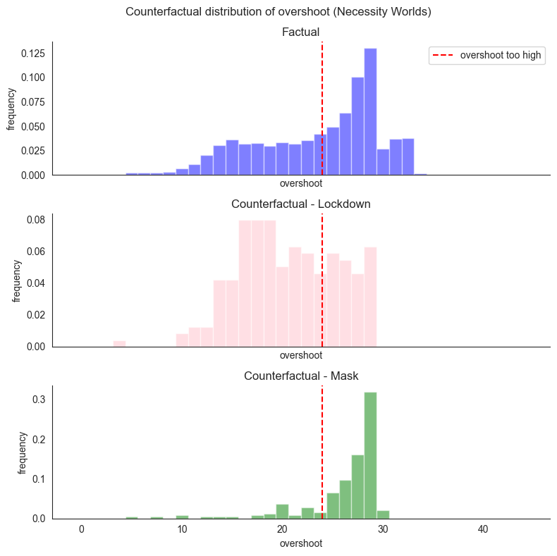
We first plot the distribution of overshoot in the factual world (indicated by world=0) and necessity counterfactual worlds (indicated by world=1) where intervened variables are set to their alternative value.

One can see how the distribution changes in the counterfactual worlds. When mask is set to 0, high overshoot is still quite likely, whereas when lockdown is set to 0, this visibly shifts the distribution towards the lower values of overhead. This agrees with the intuition that lockdown has a higher role in inducing high overshoot.

[15]:

hist_fact_nec, bin_edges, os_fact_nec, oth_fact_nec = histogram_data(
    importance_tr, mwc_imp, {}, 0
)
hist_mask_nec, bin_edges, os_mask_nec, oth_mask_nec = histogram_data(
    importance_tr,
    mwc_imp,
    {
        "__cause____antecedent_mask": 0,
        "__cause____antecedent_lockdown": 1,
        "__cause____witness_mask_efficiency": 0,
        "lockdown": 1, "mask": 1
    },
    1,
)
hist_lockdown_nec, bin_edges, os_lockdown_nec, oth_lockdown_nec = histogram_data(
    importance_tr,
    mwc_imp,
    {
        "__cause____antecedent_mask": 1,
        "__cause____antecedent_lockdown": 0,
        "__cause____witness_lockdown_efficiency": 0,
        "lockdown": 1, "mask": 1
    },
    1,
)

[16]:

fig, axes = plt.subplots(3, 1, figsize=(8, 8), sharex=True)

width = 45 / 36

axes[0].bar(
    bin_edges[:36].tolist(),
    hist_fact_nec,
    align="center",
    width=width,
    alpha=0.5,
    color="blue",
)
axes[0].axvline(x=overshoot_threshold, color="red", linestyle="--", label="overshoot too high")
axes[0].set_title("Factual")
axes[0].set_xlabel("overshoot")
axes[0].set_ylabel("frequency")
axes[0].legend()

axes[1].bar(
    bin_edges[:36].tolist(),
    hist_lockdown_nec,
    align="center",
    width=width,
    alpha=0.5,
    color="pink",
)
axes[1].axvline(x=overshoot_threshold, color="red", linestyle="--", label="overshoot too high")
axes[1].set_title("Counterfactual - Lockdown")
axes[1].set_xlabel("overshoot")
axes[1].set_ylabel("frequency")


axes[2].bar(
    bin_edges[:36].tolist(),
    hist_mask_nec,
    align="center",
    width=width,
    alpha=0.5,
    color="green",
)
axes[2].axvline(x=overshoot_threshold, color="red", linestyle="--", label="overshoot too high")
axes[2].set_title("Counterfactual - Mask")
axes[2].set_xlabel("overshoot")
axes[2].set_ylabel("frequency")

plt.suptitle("Counterfactual distribution of overshoot (Necessity Worlds)")

sns.despine()
plt.tight_layout()
plt.show()

print("Overshoot mean")
print(
    "factual: ",
    os_fact_nec.item(),
    " counterfactual mask: ",
    os_mask_nec.item(),
    " counterfactual lockdown: ",
    os_lockdown_nec.item(),
)

print("Probability of overshoot being high")
print(
    "factual: ",
    oth_fact_nec.item(),
    " counterfactual mask: ",
    oth_mask_nec.item(),
    " counterfactual lockdown: ",
    oth_lockdown_nec.item(),
)

Overshoot mean
factual:  24.302181243896484  counterfactual mask:  26.837486267089844  counterfactual lockdown:  21.276477813720703
Probability of overshoot being high
factual:  0.6021000146865845  counterfactual mask:  0.8484848737716675  counterfactual lockdown:  0.32460734248161316

The above histograms also takes into account the context that is being kept fixed. If lockdown is being intervened on, keeping lockdown_efficiency fixed would hinder the effect of the intervention.

The histograms above show three quantities:

\(P(\mathit{os} | \mathit{ld}, m)\) as the factual distribution of overshoot,
\(\sum_{w \subseteq W} P_w(w) \cdot P(\mathit{os}^w_{\mathit{ld}'} | \mathit{ld}, m)\) as counterfactual_lockdown where \(W = \{\mathit{me}\}\), and
\(\sum_{w \subseteq W} P_w(w) \cdot P(\mathit{os}^w_{\mathit{m}'} | \mathit{ld}, m)\) as counterfactual_mask where \(W = \{\mathit{le}\}\).

These distributions help in comparing how necessity interventions for the two antecedents affect the overshoot.

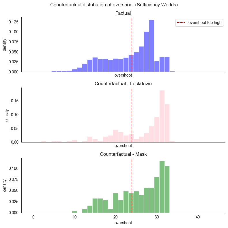
We can have similar plots for sufficiency worlds (indicated by world=2) where variables are intervened on to have their antecedent values. While this might seem redundant, this investigates probabilistically the impact of the implemented interventions: after all, it might be the case that the observed outcome is an unusual one and that usually, those interventions do not lead to the outcome of interest. The resulting plots show that when mask is set to be 1, there is a higher probability of high overshoot, but that this distribution is flatter than the distribution for lockdown being set to 1, which has higher peaks.

[17]:

hist_fact_suff, bin_edges, os_fact_suff, oth_fact_suff = histogram_data(
    importance_tr, mwc_imp, {}, 0
)
hist_mask_suff, bin_edges, os_mask_suff, oth_mask_suff = histogram_data(
    importance_tr,
    mwc_imp,
    {
        "__cause____antecedent_mask": 0,
        "__cause____antecedent_lockdown": 1,
        "__cause____witness_mask_efficiency": 0,
        "lockdown": 1, "mask": 1
    },
    2,
)
hist_lockdown_suff, bin_edges, os_lockdown_suff, oth_lockdown_suff = histogram_data(
    importance_tr,
    mwc_imp,
    {
        "__cause____antecedent_mask": 1,
        "__cause____antecedent_lockdown": 0,
        "__cause____witness_lockdown_efficiency": 0,
        "lockdown": 1, "mask": 1
    },
    2,
)

[18]:

fig, axes = plt.subplots(3, 1, figsize=(8, 8), sharex=True)


axes[0].bar(
    bin_edges[:36].tolist(),
    hist_fact_suff,
    align="center",
    width=width,
    alpha=0.5,
    color="blue",
)
axes[0].axvline(x=overshoot_threshold, color="red", linestyle="--", label="overshoot too high")
axes[0].set_title("Factual")
axes[0].set_xlabel("overshoot")
axes[0].set_ylabel("density")
axes[0].legend()

axes[1].bar(
    bin_edges[:36].tolist(),
    hist_lockdown_suff,
    align="center",
    width=width,
    alpha=0.5,
    color="pink",
)
axes[1].axvline(x=overshoot_threshold, color="red", linestyle="--", label="overshoot too high")
axes[1].set_title("Counterfactual - Lockdown")
axes[1].set_xlabel("overshoot")
axes[1].set_ylabel("density")

axes[2].bar(
    bin_edges[:36].tolist(),
    hist_mask_suff,
    align="center",
    width=width,
    alpha=0.5,
    color="green",
)
axes[2].axvline(x=overshoot_threshold, color="red", linestyle="--", label="overshoot too high")
axes[2].set_title("Counterfactual - Mask")
axes[2].set_xlabel("overshoot")
axes[2].set_ylabel("density")


plt.suptitle("Counterfactual distribution of overshoot (Sufficiency Worlds)")

sns.despine()
plt.tight_layout()
plt.show()

print("Overshoot mean")
print(
    "factual: ",
    os_fact_suff.item(),
    " counterfactual mask: ",
    os_mask_suff.item(),
    " counterfactual lockdown: ",
    os_lockdown_suff.item(),
)

print("Probability of overshoot being high")
print(
    "factual: ",
    oth_fact_suff.item(),
    " counterfactual mask: ",
    oth_mask_suff.item(),
    " counterfactual lockdown: ",
    oth_lockdown_suff.item(),
)

Overshoot mean
factual:  24.302181243896484  counterfactual mask:  26.423648834228516  counterfactual lockdown:  27.30312728881836
Probability of overshoot being high
factual:  0.6021000146865845  counterfactual mask:  0.6717171669006348  counterfactual lockdown:  0.717277467250824

The histograms above show three quantities:

\(P(\mathit{os} | \mathit{ld}, m)\) as the factual distribution of overshoot,
\(\sum_{w \subseteq W} P_w(w) \cdot P(\mathit{os}^w_{\mathit{ld}} | \mathit{ld}, m)\) as counterfactual_lockdown where \(W = \{\mathit{me}\}\), and
\(\sum_{w \subseteq W} P_w(w) \cdot P(\mathit{os}^w_{\mathit{m}} | \mathit{ld}, m)\) as counterfactual_mask where \(W = \{\mathit{le}\}\).

Again, these distributions help in comparing how sufficiency interventions for the two antecedents affect the overshoot.

We can also combine samples from both sufficiency and necessity worlds to focus on a context-sensitive counterpart of the joint probability of necessity and sufficiency directly (see the previous tutorial for more explanation). We first visualize samples where only lockdown is considered as an intervention. Then we analyze masking as an intervention.

[19]:

# Collecting samples for joint distribution of overshoot under necessity and sufficiency interventions on lockdown
masks = {
        "__cause____antecedent_mask": 1,
        "__cause____antecedent_lockdown": 0,    # Intervening only on lockdown
        "__cause____witness_lockdown_efficiency": 0, # Excluding lockdown efficiency fron the context candidates
        "lockdown": 1, "mask": 1 # Conditioning on lockdown and masking being imposed in factual world
    }
with mwc_imp:
    data_nec = gather(
        importance_tr.nodes["overshoot"]["value"],
        IndexSet(**{"lockdown": {1}, "mask": {1}}),
    )

    data_suff = gather(
        importance_tr.nodes["overshoot"]["value"],
        IndexSet(**{"lockdown": {2}, "mask": {2}}),
    )


    mask_tensor = torch.ones(
        importance_tr.nodes["__cause____antecedent_mask"]["value"].shape
    ).bool()
    for key, val in masks.items():
        mask_tensor = mask_tensor & (importance_tr.nodes[key]["value"] == val)

    data_suff = data_suff.squeeze()[torch.nonzero(mask_tensor.squeeze())]
    data_nec = data_nec.squeeze()[torch.nonzero(mask_tensor.squeeze())]

a = torch.transpose(torch.vstack((data_nec.squeeze(), data_suff.squeeze())), 0, 1) # Joint distribution
hist_lockdown_2d, rough = torch.histogramdd(a, bins=[36, 36], density=True, range=[0.0, 45.0, 0.0, 45.0])
pr_lockdown = (hist_lockdown_2d[:16, 16:].sum()/hist_lockdown_2d.sum())


# Collecting samples for joint distribution of overshoot under necessity and sufficiency interventions on mask
masks = {
        "__cause____antecedent_mask": 0,
        "__cause____antecedent_lockdown": 1,    # Intervening only on mask
        "__cause____witness_mask_efficiency": 0,    # Excluding mask efficiency fron the context candidates
        "lockdown": 1, "mask": 1    # Conditioning on lockdown and masking being imposed in factual world
    }
with mwc_imp:
    data_nec = gather(
        importance_tr.nodes["overshoot"]["value"],
        IndexSet(**{"lockdown": {1}, "mask": {1}}),
    )

    data_suff = gather(
        importance_tr.nodes["overshoot"]["value"],
        IndexSet(**{"lockdown": {2}, "mask": {2}}),
    )

    mask_tensor = torch.ones(
        importance_tr.nodes["__cause____antecedent_mask"]["value"].shape
    ).bool()
    for key, val in masks.items():
        mask_tensor = mask_tensor & (importance_tr.nodes[key]["value"] == val)

    data_suff = data_suff.squeeze()[torch.nonzero(mask_tensor.squeeze())]
    data_nec = data_nec.squeeze()[torch.nonzero(mask_tensor.squeeze())]

a = torch.transpose(torch.vstack((data_nec.squeeze(), data_suff.squeeze())), 0, 1) # Joint distribution
hist_mask_2d, _ = torch.histogramdd(a, bins = [36, 36], density=True, range=[0.0, 45.0, 0.0, 45.0])
pr_mask = (hist_mask_2d[:16, 16:].sum()/hist_mask_2d.sum())

[20]:

fig, axs = plt.subplots(1, 2, figsize=(16, 8))

# Heatmap for counterfactual lockdown
ax = axs[0]
hist_lockdown_2d = hist_lockdown_nec.unsqueeze(1) * hist_lockdown_suff.unsqueeze(0)
im = ax.imshow(hist_lockdown_2d, cmap="viridis")
ax.set(xticks=range(0, 36, 2), xticklabels=bin_edges[0:36:2].tolist())
ax.set(yticks=range(0, 36, 2), yticklabels=bin_edges[0:36:2].tolist())
ax.set(
    xlabel="Overshoot under sufficiency Intervention",
    ylabel="Overshoot under necessity Intervention",
    title="Overshoot in counterfactual lockdown",
)
ax.axvline(x=(overshoot_threshold) * 36 / 45, color="red", linestyle="--", label="Overshoot too high")
ax.axhline(y=(overshoot_threshold) * 36 / 45, color="red", linestyle="--")
ax.axvline(x=(os_lockdown_suff) * 36 / 45, color="white", linestyle="--", label="Mean Overshoot")
ax.axhline(y=(os_lockdown_nec) * 36 / 45, color="white", linestyle="--")
ax.legend(loc="upper left")
ax.text(21, 2, 'pr(lockdown has causal role \n over high overshoot): %.4f' % pr_lockdown.item(), color="white")


cbar1 = fig.colorbar(im, ax=ax, orientation="vertical", fraction=0.046, pad=0.04)
cbar1.set_label("density")

ax = axs[1]
hist_mask_2d = hist_mask_nec.unsqueeze(1) * hist_mask_suff.unsqueeze(0)
im = ax.imshow(hist_mask_2d, cmap="viridis")
ax.set(xticks=range(0, 36, 2), xticklabels=bin_edges[0:36:2].tolist())
ax.set(yticks=range(0, 36, 2), yticklabels=bin_edges[0:36:2].tolist())
ax.set(
    xlabel="Overshoot under sufficiency intervention",
    ylabel="Overshoot under necessity intervention",
    title="Overshoot in counterfactual mask",
)
ax.axvline(x=(overshoot_threshold) * 36 / 45, color="red", linestyle="--", label="Overshoot too high")
ax.axhline(y=(overshoot_threshold) * 36 / 45, color="red", linestyle="--")
ax.axvline(x=(os_mask_suff) * 36 / 45, color="white", linestyle="--", label="Mean Overshoot")
ax.axhline(y=(os_mask_nec) * 36 / 45, color="white", linestyle="--")
ax.text(21, 2, 'pr(masking has causal role \n over high overshoot): %.4f' % pr_mask.item(), color="white")
ax.legend(loc="upper left")

cbar2 = fig.colorbar(im, ax=ax, orientation="vertical", fraction=0.046, pad=0.04)
cbar2.set_label("density")

sns.despine()
plt.tight_layout()
plt.suptitle("Counterfactual heatmap of overshoot under necessity and sufficiency interventions")
plt.show()

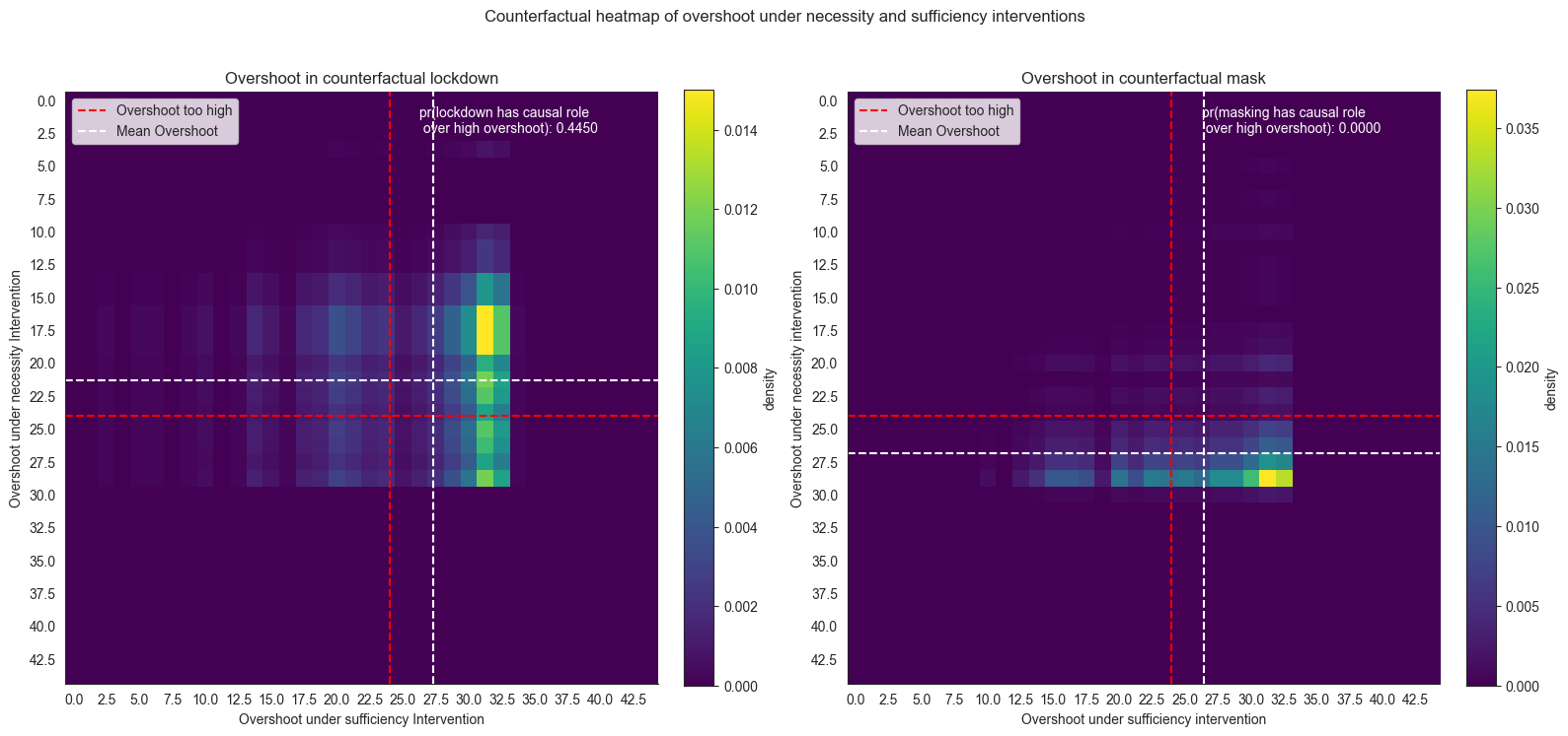
The above heatmaps plot the joint distributions arising from necessity and sufficient interventions:

\(\sum_{w \subseteq W} P_w(w) \cdot P(\mathit{os}^w_{\mathit{ld}}, \mathit{os}^w_{\mathit{ld}'}|\mathit{ld, m})\) where \(W = \{\mathit{me}\}\) and
\(\sum_{w \subseteq W} P_w(w) \cdot P(\mathit{os}^w_{\mathit{m}}, \mathit{os}^w_{\mathit{m}'}|\mathit{ld, m})\), where \(W = \{\mathit{le}\}\).

The key to interpreting this heatmap is the fact that we plot two different counterfactual distributions against each other here. Along the x-axis we show what overshoot a model expects under the sufficiency intervention. And here, we see that for both interventions the model expects most of the density to lie above the overshoot threshold (red). So both intereventions are, approximately, sufficient. On the y-axis, however, we show the counterfactual distribution in the necessity world, where the intervention does not take place. Note that the scale starts in the upper left corner. This means that the higher the density mass is on the plot, the lower is the expected overshoot without that intervention, i.e. “the more necessary” a given intervention is for the outcome. Here, only lockdown seems to play a necessary role. Ideally, however, we are interested in whether an intervention is both necessary and sufficient, the probablity of which is the proportion of density mass in the upper-right quandrant determined by the dashed red lines. It is evident from the plot above that the counterfactual for lockdown has more probability mass in the top right quadrant (low overshoot in the necessity world and high overshoot in the sufficient world). This gives us a clearer picture into why lockdown has higher causal role in the overshoot being too high as compared to masking.

`Looking into different contexts for curious readers <#toc0_>`__¶

SearchForExplanation allows the users to perform an even finer-grained analysis by visualizing distributions of random variables when different contexts are kept fixed in the model. To illustrate this, we consider the following two scenarios:

Intervene on lockdown=1 while keeping mask_efficiency fixed (or not).
Intervene on mask=1 while keeping lockdown_efficiency fixed (or not).

The key motivation for looking into this is the intuition that there is some part of the actual context in which removing lockdown would significantly lower the overshoot, whereas there is no corresponding part of the actual context in which removing masking would lead to lower overshoot - which is the core of the asymmetry between the two interventions in our example.

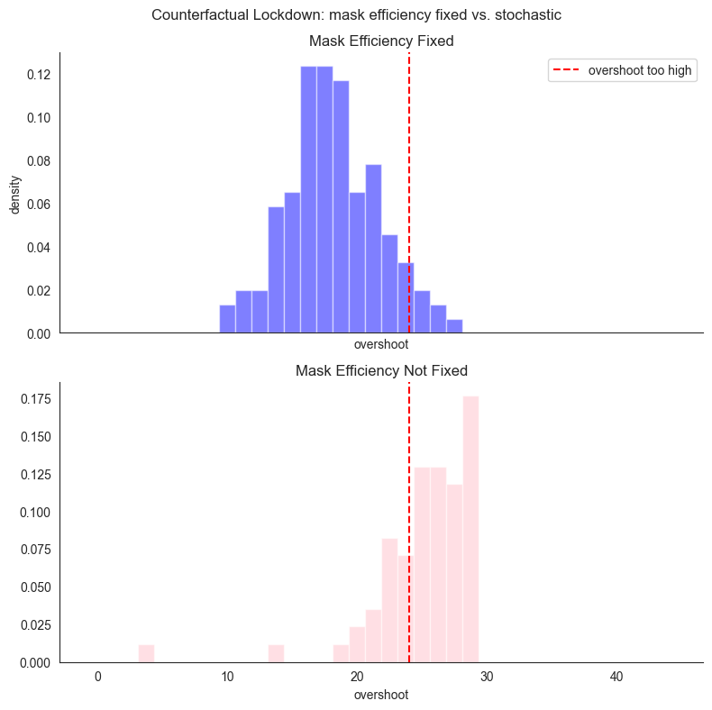
We first intervene on lockdown being 1 and analyze how the distribution of overshoot changes as we keep the mask_efficiency fixed (or not).

[21]:

hist_lockdown_fix, bin_edges, os_lockdown_fix, oth_lockdown_fix = histogram_data(
    importance_tr,
    mwc_imp,
    {
        "__cause____antecedent_mask": 1,
        "__cause____antecedent_lockdown": 0,
        "__cause____witness_lockdown_efficiency": 0,
        "__cause____witness_mask_efficiency": 1,
        "lockdown": 1, "mask": 1
    },
    1,
)
hist_lockdown_notfix, bin_edges, os_lockdown_notfix, oth_lockdown_notfix = (
    histogram_data(
        importance_tr,
        mwc_imp,
        {
            "__cause____antecedent_mask": 1,
            "__cause____antecedent_lockdown": 0,
            "__cause____witness_lockdown_efficiency": 0,
            "__cause____witness_mask_efficiency": 0,
            "lockdown": 1, "mask": 1
        },
        1,
    )
)

[22]:

fig, axes = plt.subplots(2, 1, figsize=(8, 8), sharex=True)

axes[0].bar(
    bin_edges[:36].tolist(),
    hist_lockdown_fix,
    align="center",
    width=width,
    alpha=0.5,
    color="blue",
)
axes[0].axvline(x=overshoot_threshold, color="red", linestyle="--", label="overshoot too high")
axes[0].set_title("Mask Efficiency Fixed")
axes[0].set_xlabel("overshoot")
axes[0].set_ylabel("density")
axes[0].legend()

axes[1].bar(
    bin_edges[:36].tolist(),
    hist_lockdown_notfix,
    align="center",
    width=width,
    alpha=0.5,
    color="pink",
)
axes[1].axvline(x=overshoot_threshold, color="red", linestyle="--", label="overshoot too high")
axes[1].set_title("Mask Efficiency Not Fixed")
axes[1].set_xlabel("overshoot")


plt.suptitle("Counterfactual Lockdown: mask efficiency fixed vs. stochastic")

sns.despine()
plt.tight_layout()
plt.show()

print("Overshoot mean")
print(
    "mask_efficiency fixed: ",
    os_lockdown_fix.item(),
    " mask_efficiency not fixed: ",
    os_lockdown_notfix.item(),
)

print("Probability of overshoot being high")
print(
    "mask_efficiency fixed: ",
    oth_lockdown_fix.item(),
    " mask_efficiency not fixed: ",
    oth_lockdown_notfix.item(),
)

Overshoot mean
mask_efficiency fixed:  18.7790470123291  mask_efficiency not fixed:  25.793893814086914
Probability of overshoot being high
mask_efficiency fixed:  0.08130080997943878  mask_efficiency not fixed:  0.7647058963775635

The above histogram plots the following distributions:

mask_efficiency fixed: \(P( \mathit{os}^{\mathit{me}}_{\mathit{ld}'} | \mathit{ld}, m)\)
mask_efficiency not fixed: \(P( \mathit{os}_{\mathit{ld}'} | \mathit{ld}, m)\)

The plot clearly shows that depending on the fact that mask_efficiency was kept fixed on the factual value or not, the overshoot variable changes. Crucially, if we keep the mask efficiency at the actual value, the probability of the overshoot being too high drops down to \(\approx 0.08\).

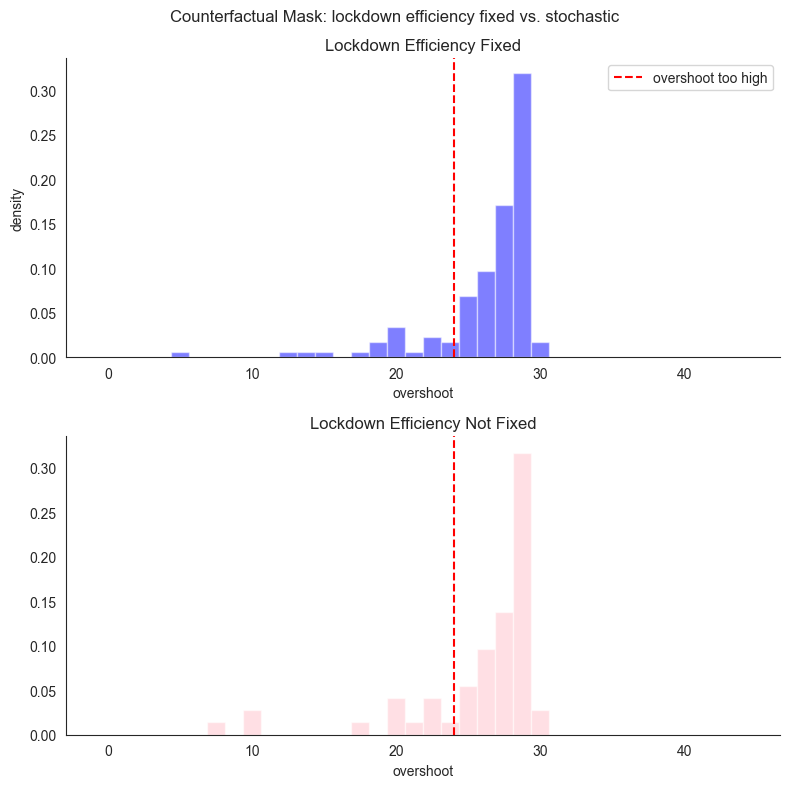
We then run an analogous analysis for masking - we intervene on mask being 1 and analyze how the distribution of overshoot change as we keep the lockdown_efficiency fixed or not.

[23]:

hist_mask_fix, bin_edges, os_mask_fix, oth_mask_fix = histogram_data(
    importance_tr,
    mwc_imp,
    {
        "__cause____antecedent_mask": 0,
        "__cause____antecedent_lockdown": 1,
        "__cause____witness_mask_efficiency": 0,
        "__cause____witness_lockdown_efficiency": 1,
        "lockdown": 1, "mask": 1
    },
    1,
)
hist_mask_notfix, bin_edges, os_mask_notfix, oth_mask_notfix = histogram_data(
    importance_tr,
    mwc_imp,
    {
        "__cause____antecedent_mask": 0,
        "__cause____antecedent_lockdown": 1,
        "__cause____witness_mask_efficiency": 0,
        "__cause____witness_lockdown_efficiency": 0,
        "lockdown": 1, "mask": 1
    },
    1,
)

[24]:

fig, axes = plt.subplots(2, 1, figsize=(8, 8), sharey=True)


axes[0].bar(
    bin_edges[:36].tolist(),
    hist_mask_fix,
    align="center",
    width=width,
    alpha=0.5,
    color="blue",
)
axes[0].axvline(x=overshoot_threshold, color="red", linestyle="--", label="overshoot too high")
axes[0].set_title("Lockdown Efficiency Fixed")
axes[0].set_xlabel("overshoot")
axes[0].set_ylabel("density")
axes[0].legend()

axes[1].bar(
    bin_edges[:36].tolist(),
    hist_mask_notfix,
    align="center",
    width=width,
    alpha=0.5,
    color="pink",
)
axes[1].axvline(x=overshoot_threshold, color="red", linestyle="--", label="overshoot too high")
axes[1].set_title("Lockdown Efficiency Not Fixed")
axes[1].set_xlabel("overshoot")


plt.suptitle("Counterfactual Mask: lockdown efficiency fixed vs. stochastic")
sns.despine()
plt.tight_layout()
plt.show()


print("Overshoot mean")
print(
    "lockdown_efficiency fixed: ",
    os_mask_fix.item(),
    " lockdown_efficiency not fixed: ",
    os_mask_notfix.item(),
)

print("Probability of overshoot being high")
print(
    "lockdown_efficiency fixed: ",
    oth_mask_fix.item(),
    " lockdown_efficiency not fixed: ",
    oth_mask_notfix.item(),
)

Overshoot mean
lockdown_efficiency fixed:  27.030378341674805  lockdown_efficiency not fixed:  26.37188148498535
Probability of overshoot being high
lockdown_efficiency fixed:  0.8642857074737549  lockdown_efficiency not fixed:  0.8103448152542114

Similar to the earlier histogram, the above plot shows the following distributions:

lockdown_efficiency fixed: \(P( \mathit{os}^{\mathit{le}}_{\mathit{m}'} | \mathit{ld}, m)\)
lockdown_efficiency not fixed: \(P( \mathit{os}_{\mathit{m}'} | \mathit{ld}, m)\)

The plot clearly shows that lockdown_efficiency as a context has little effect on how intervening on mask affects overshoot. Again, crucially, whichever context setting we choose here, withdrawing the masking policy does not radically change the fact that the overshoot is still very likely to be too high.

`Conclusions <#toc0_>`__¶

SearchForExplanation can be used in any ChiRho causal model to investigate the causal role of variables of interest in outome variables having the values that they do in particular runs. This is achieved by transforming the causal model into one that allows us to investigate multiple causal settings with “necessity” and “sufficiency” interventions and their impact on the outcome variable across different possible worlds. Looking back at the heatmap, “Counterfactual heatmap of overshoot under necessity and sufficiency interventions” with the accompanying explanation illustrates how paying attention to both conjoining sufficiency and necessity and to searching through actual contexts to be fixed allows us to break the prima facie symmetries which makes the usual but-for analysis blind to such a fine-grained analysis. Moreover, the obtained samples can be used to answer more specific causal queries if need be.

A practical policy-making implication is that developing causal models for problems at hand and employing a strategy analogous to the one discussed in this notebook is a promising strategy for a fine-grained and probabilistically aware responsibility attribution.