Estimating the causal effects of drug treatment on gene expression¶

Outline¶

Dev Setup
Understanding the mechanism of action of a drug using causal inference
Goal: Understand the effects that the cancer drug candidate Pracinostat SB939 has on other target genes
- Exploratory data analysis
Causal Probabilistic Program
Computing causal queries
- Causal Query: Average treatment effect (ATE)
- Causal Query: Conditional average treatment effect (CATE)
References

Dev setup¶

Here, we install the necessary Pytorch, Pyro, and ChiRho dependencies for this example.

[1]:

%load_ext autoreload
%autoreload 2

[2]:

%%capture
!pip install scanpy pybiomart numpy==1.23 seaborn==0.12.2 # add single cell dependencies

[3]:

import os
import math
import numpy as np
import scipy.sparse
import pandas as pd
import scanpy as sc
from scipy.stats import pearsonr
import matplotlib.pyplot as plt
import seaborn as sns
import pyro
from pyro.infer.autoguide import AutoNormal
from pyro.nn import PyroModule
import pyro.distributions as dist
from IPython.display import Image
import torch

from chirho.counterfactual.handlers import MultiWorldCounterfactual
from chirho.indexed.ops import IndexSet, gather
from chirho.interventional.handlers import do
from chirho.observational.handlers import condition

pyro.clear_param_store()
pyro.set_rng_seed(1234)
pyro.settings.set(module_local_params=True)

sns.set_style("white")

Understanding the mechanism of action of a drug using causal inference¶

Experimental design¶

We analyze the SciPlex3 dataset from Srivatsan (2020), which uses “nuclear hashing” to measure global transcriptional responses to over 4,000 unique perturbations at single-cell resolution. This hashing technique is summarized below:

[4]:

# Figure 1B from Srivatsan (2020)
# Cells corresponding to different perturbations are lysed in-well, their nuclei labeled with well-specific “hash” oligos,
# followed by fixation, pooling, and sci-RNA-seq.
Image('./figures/sciplex_fig1b.png', width=500)

[4]:

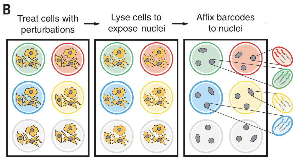
Using this experimental setup, Srivatsan (2020) profiled the effects of 188 drugs on three different cancer cell types: MCF7, K562, and A549. Each cell in this dataset is unperturbed (Vehicle) or randomly treated with a drug from a library of 188 drug perburbations (product_name) at 4 different dosages (dose): $10^1, 10^2, 10^3, 10^4$ nM. After 24hrs, the expressions of each gene are measured. Hence, apart from technical confounders such as batch effects, the differences in gene expression between the treated and untreated cells are caused by the drug perturbation. Figure 3A summarizes this combinatorial experimental design.

[5]:

Image('./figures/sciplex_fig3a.png', width=1000)

[5]:

Data ingestion¶

scPerturb (https://github.com/sanderlab/scPerturb/) provides pre-processed single-cell RNA seq datasets, including the SciPlex3 dataset from Srivatsan (2020). Unfortunately, there is an issue in scPerturb with processing the SciPlex3 dataset (https://github.com/sanderlab/scPerturb/issues/7). We fix the bug in their script (https://github.com/sanderlab/scPerturb/blob/master/dataset_processing/SrivatsanTrapnell2020.py) below.

[6]:

# Download raw data if doesn't already exist
if os.path.exists("SrivatsanTrapnell2020_sciplex3_debugged.h5"):
    anndata = sc.read_h5ad("SrivatsanTrapnell2020_sciplex3_debugged.h5")
else:
    # Download and unzip 3 files files from here:
    # https://www.ncbi.nlm.nih.gov/geo/query/acc.cgi?acc=GSM4150378
    # (1) GSM4150378_sciPlex3_A549_MCF7_K562_screen_UMI.count.matrix.gz
    # (2) GSM4150378_sciPlex3_A549_MCF7_K562_screen_gene.annotations.txt.gz
    # (3) GSM4150378_sciPlex3_pData.txt.gz

    # Cach raw zip files
    os.system(
        "wget -c https://ftp.ncbi.nlm.nih.gov/geo/samples/GSM4150nnn/GSM4150378/suppl/GSM4150378_sciPlex3_A549_MCF7_K562_screen_UMI.count.matrix.gz"
    )
    os.system(
        "wget -c https://ftp.ncbi.nlm.nih.gov/geo/samples/GSM4150nnn/GSM4150378/suppl/GSM4150378_sciPlex3_A549_MCF7_K562_screen_gene.annotations.txt.gz"
    )

    os.system(
        "wget -c https://ftp.ncbi.nlm.nih.gov/geo/samples/GSM4150nnn/GSM4150378/suppl/GSM4150378_sciPlex3_pData.txt.gz"
    )

    # unzip files
    os.system("gunzip GSM4150378_sciPlex3_A549_MCF7_K562_screen_UMI.count.matrix.gz")
    os.system("gunzip GSM4150378_sciPlex3_A549_MCF7_K562_screen_gene.annotations.txt.gz")
    os.system("gunzip GSM4150378_sciPlex3_pData.txt.gz")

    var = pd.read_csv(
        "GSM4150378_sciPlex3_A549_MCF7_K562_screen_gene.annotations.txt",
        sep=" ",
    )
    var.columns = ["gene_id", "gene_name"]

    var = var.set_index("gene_name")

    obs2 = pd.read_csv("GSM4150378_sciPlex3_pData.txt", sep=" ")

    UMI_counts = pd.read_csv(
        "GSM4150378_sciPlex3_A549_MCF7_K562_screen_UMI.count.matrix", sep="\t", header=None
    )

    X = scipy.sparse.csr_matrix(
        (UMI_counts[2], (UMI_counts[1] - 1, UMI_counts[0] - 1)), shape=(len(obs2), len(var))
    )  # this may crash your kernel

    UMI_counts = None  # save on memory
    anndata = sc.AnnData(X, obs=obs2, var=var)

    # reform var
    anndata.var.index = anndata.var.index.rename("gene_symbol")
    anndata.var["ensembl_gene_id"] = [x.split(".")[0] for x in anndata.var["gene_id"]]
    anndata.obs["dose_unit"] = "nM"
    anndata.obs["celltype"] = [
        "alveolar basal epithelial cells"
        if line == "A549"
        else "mammary epithelial cells"
        if line == "MCF7"
        else "lymphoblasts"
        if line == "K562"
        else "None"
        for line in anndata.obs.cell_type
    ]
    anndata.obs["disease"] = [
        "lung adenocarcinoma"
        if line == "A549"
        else "breast adenocarcinoma"
        if line == "MCF7"
        else "chronic myelogenous leukemia"
        if line == "K562"
        else "None"
        for line in anndata.obs.cell_type
    ]
    anndata.write("SrivatsanTrapnell2020_sciplex3_debugged.h5")

/opt/homebrew/anaconda3/envs/basis/lib/python3.10/site-packages/anndata/_core/anndata.py:1840: UserWarning: Variable names are not unique. To make them unique, call `.var_names_make_unique`.
  utils.warn_names_duplicates("var")

[7]:

# Data is 12GB
!du -sh *h5

 12G    SrivatsanTrapnell2020_sciplex3_debugged.h5

Data preprocessing¶

We preprocess the data as follows: - Filter out cells that have unknown cell type - Only include measurements at the 24hr timepoint (retains ~90% of the dataset) - Restrict to human genes since all cells are from human cell lines - Filter out genes that are expressed in fewer than 10 cells - Filter out cells that have fewer than 200 expressed genes - Mitochondrial ratio quality (based on visual inspection) - Read counts

[8]:

# Remove unknown cell types
anndata = anndata[~anndata.obs['cell_type'].isnull()]

# Filter out to only 24hr observations (~90% of the data remains)
anndata = anndata[anndata.obs['time_point'] == 24]

# Restrict to genes in human genome
annot = sc.queries.biomart_annotations(
    "hsapiens", ["ensembl_gene_id", "hgnc_symbol"]
)
annot = annot.dropna()
anndata = anndata[:, anndata.var['ensembl_gene_id'].isin(annot['ensembl_gene_id'].values)]

# Filter out genes that are expressed in less than 10 cells
sc.pp.filter_genes(anndata, min_cells=10)

# Filter out cells that express less than 200 genes
sc.pp.filter_cells(anndata, min_genes=200)

/opt/homebrew/anaconda3/envs/basis/lib/python3.10/site-packages/scanpy/preprocessing/_simple.py:251: ImplicitModificationWarning: Trying to modify attribute `.var` of view, initializing view as actual.
  adata.var['n_cells'] = number
/opt/homebrew/anaconda3/envs/basis/lib/python3.10/site-packages/anndata/_core/anndata.py:1840: UserWarning: Variable names are not unique. To make them unique, call `.var_names_make_unique`.
  utils.warn_names_duplicates("var")
/opt/homebrew/anaconda3/envs/basis/lib/python3.10/site-packages/anndata/_core/anndata.py:1840: UserWarning: Variable names are not unique. To make them unique, call `.var_names_make_unique`.
  utils.warn_names_duplicates("var")
/opt/homebrew/anaconda3/envs/basis/lib/python3.10/site-packages/anndata/_core/anndata.py:1840: UserWarning: Variable names are not unique. To make them unique, call `.var_names_make_unique`.
  utils.warn_names_duplicates("var")

[9]:

# Trim outliers by
# 1. Mitochondrial ratio quality
# 2. total read counts
# 3. number of genes per cell
anndata.var["mt"] = anndata.var_names.str.startswith("MT-")
sc.pp.calculate_qc_metrics(
    anndata, qc_vars=["mt"], percent_top=None, log1p=False, inplace=True
)

anndata.var_names_make_unique()
# Quality plots to identify outliers
sc.pl.violin(
    anndata,
    ["n_genes_by_counts", "total_counts", "pct_counts_mt"],
    jitter=0.3,
    multi_panel=True,
    stripplot=False
)

[10]:

# define outliers and do the filtering for the sciplex data
# with arbitrary cutoffs
anndata.obs['outlier_mt'] = anndata.obs.pct_counts_mt > 60
anndata.obs['outlier_total'] = anndata.obs.total_counts > 20000
anndata.obs['outlier_ngenes'] = anndata.obs.n_genes_by_counts > 6000

print('%u cells with high %% of mitochondrial genes' % (sum(anndata.obs['outlier_mt'])))
print('%u cells with large total counts' % (sum(anndata.obs['outlier_total'])))
print('%u cells with large number of genes' % (sum(anndata.obs['outlier_ngenes'])))

anndata = anndata[~anndata.obs['outlier_mt'], :]
anndata = anndata[~anndata.obs['outlier_total'], :]
anndata = anndata[~anndata.obs['outlier_ngenes'], :]
sc.pp.filter_genes(anndata, min_cells=1)

655 cells with high % of mitochondrial genes
2713 cells with large total counts
1481 cells with large number of genes

/opt/homebrew/anaconda3/envs/basis/lib/python3.10/site-packages/scanpy/preprocessing/_simple.py:251: ImplicitModificationWarning: Trying to modify attribute `.var` of view, initializing view as actual.
  adata.var['n_cells'] = number

Goal: Understand the effects that the cancer drug candidate Pracinostat SB939 has on other target genes¶

We choose a particular drug (Pracinostat (SB939)), which is currently in a Phase II clinical trial for treating T cell lymphoma. We start our analysis by looking at several summary statistics and visualizations of this drug. Then, we use ChiRho to estimate the causal effect of this drug on gene expression levels.

Below we look at which pathway Pracinostat (SB939) targets.

[11]:

anndata.obs[anndata.obs.product_name.str.contains("Pracin")][['target']].drop_duplicates().reset_index(drop=True)

[11]:

	target
0	HDAC

Histone deacetylase (HDAC) inhibitors are anti-cancer agents that can induce death, apoptosis, and cell cycle arrest in cancer cells Kim (2011). HDAC inhibitors have been shown to modify the activity of many transcription factors. Some of these include NCOA3, MYB, E2F1, KLF1, FEN1, GATA1, HNF4A, XRCC6, NFκB, PCNA, TP53, RB1, Runx, SF1 Sp3, STAT, GTF2E1, TCF7L2, YY1 (Drummond 2005, Yang 2007). We focus on modeling the changes in expression of genes associated with these transcription factors in response to Pracinostat (target_genes). We would like to understand which of the genes in target_genes are (1) most affected by Pracinostat, (2) upregulated or downregulated, and (3) have effects that vary across different cell types.

[12]:

drug_target = "Pracinostat (SB939)"
drug_data = anndata[anndata.obs.product_name.str.contains("Pracinostat|Vehi")]
anndata = None # save on memory

To pick the target set of genes, we select from a combination of different gene sets. We select SIRT2 in target_genes below since it is a direct HDAC inhibitor, and validated as being upregulated by HDAC inhibitor drugs in Srivatsan (2020). We also select a list of the genes from Drummond (2005) and Yang (2007) that represent genes associated with transcription factors reported to be downstream of HDAC inhibitors. Finally, we use the Cistrome Data Browser (an epigenetic profile database) to select the “top five genes” potentially regulated by the enhancers. We select these “top 5 genes” by looking at the enhancers with the highest enriched H3K27ac signals for each cell line (based on ChIP-seq). This choice is motivated by the fact that an HDAC inhibitor will change the global acetylation levels. We assume that the top genes marked by H3K27ac are potentially regulated by the enhancers with the highest enriched H3K27ac signals in the same cell lines.

[13]:

# Genes from https://en.wikipedia.org/wiki/Histone_deacetylase#HDAC_inhibitors
wiki_genes = [
    'NCOA3', 'MYB', 'E2F1', 'KLF1', 'FEN1', 'GATA1', 'HNF4A', 'XRCC6', 'NFKB1', 'PCNA', 'TP53', 'RB1', 'RUNX1', 'SF1', 'SP3', 'STAT1', 'GTF2E1', 'TCF7L2', 'YY1', 'SIRT2'
]

# http://cistrome.org/db/#/
# Search "h3k27ac" and input each cell type into "Biological Sources" field
# Select first study and top 5 from "Get Putative Targets"
chipseq_a549_targets = [
    "PSME2", "RNF31", "EMC9", "METTL26", "NPY4R"
]

chipseq_k562_targets = [
    "ZBTB4", "POLR2A", "UFD1", "CDC45", 'SLC9A5' # SLC35G6 not in dataset
]

chipseq_mcf7_targets = [
    "IDI1", "MAFG", "LAMTOR2", "UBQLN4", "RPS2"
]

# Add SIRT2 gene to validate against Srivatsan (2020)
target_genes = wiki_genes + chipseq_a549_targets + chipseq_k562_targets + chipseq_mcf7_targets + ['SIRT2']

Exploratory data analysis¶

[14]:

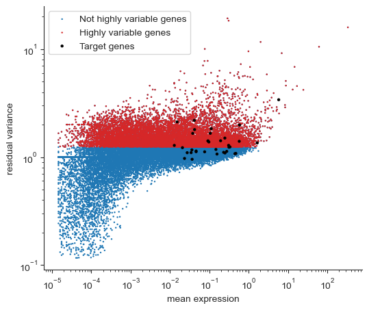
# Use pearson residuals for better gene visualization
# see https://genomebiology.biomedcentral.com/articles/10.1186/s13059-021-02451-7
sc.experimental.pp.highly_variable_genes(
    drug_data, flavor="pearson_residuals", n_top_genes=10000
)

/opt/homebrew/anaconda3/envs/basis/lib/python3.10/site-packages/scanpy/experimental/pp/_highly_variable_genes.py:67: UserWarning: Received a view of an AnnData. Making a copy.
  view_to_actual(adata)

[15]:

fig, ax = plt.subplots(1, figsize=(6, 5))

hvgs = drug_data.var["highly_variable"]

ax.scatter(
    drug_data.var["mean_counts"], drug_data.var["residual_variances"], s=3, edgecolor="none",
    label='Not highly variable genes'
)
ax.scatter(
    drug_data.var["mean_counts"][hvgs],
    drug_data.var["residual_variances"][hvgs],
    c="tab:red",
    label="Highly variable genes",
    s=3,
    edgecolor="none",
)
ax.scatter(
    drug_data.var["mean_counts"][target_genes],
    drug_data.var["residual_variances"][target_genes],
    c="k",
    label="Target genes",
    s=10,
    edgecolor="none",
)

ax.set_xscale("log")
ax.set_xlabel("mean expression")
ax.set_yscale("log")
ax.set_ylabel("residual variance")
ax.spines["right"].set_visible(False)
ax.spines["top"].set_visible(False)
ax.yaxis.set_ticks_position("left")
ax.xaxis.set_ticks_position("bottom")

ax.legend()

[15]:

<matplotlib.legend.Legend at 0x171b3fd90>

[16]:

# Filter to highly variable genes
drug_data = drug_data[:, drug_data.var["highly_variable"]]

# Remove low variance genes in target_genes based on pearson residuals
target_genes = np.intersect1d(target_genes, drug_data.var_names[drug_data.var.highly_variable])
# target_genes = np.array(drug_data.var_names[drug_data.var.highly_variable])

Let’s look at how each cell clusters based on cell type and if the cell was given the drug or not using a Uniform Manifold Approximation and Projection (UMAP) embedding of the highly variable genes.

[17]:

# The UMAP function does a visualization using 'X' in the anndata object
# We save the raw counts for later use
drug_data.layers["raw"] = drug_data.X.copy()

# Now, 'X' refers to pearson residuals
sc.experimental.pp.normalize_pearson_residuals(drug_data)

# Log1p normalize of the data (used for UMAP visual)
drug_data.layers["log1p"] = np.log1p(
    sc.pp.normalize_total(drug_data, inplace=False)["X"]
)

sc.pp.neighbors(drug_data, n_neighbors=30, n_pcs=30)
sc.tl.umap(drug_data)

/opt/homebrew/anaconda3/envs/basis/lib/python3.10/site-packages/scanpy/preprocessing/_normalization.py:197: UserWarning: Some cells have zero counts
  warn(UserWarning('Some cells have zero counts'))

WARNING: You’re trying to run this on 10000 dimensions of `.X`, if you really want this, set `use_rep='X'`.
         Falling back to preprocessing with `sc.pp.pca` and default params.

/var/folders/1n/rv21b_n10gx0tp5_zz33z7qc0000gn/T/ipykernel_54317/397955117.py:9: RuntimeWarning: invalid value encountered in log1p
  drug_data.layers["log1p"] = np.log1p(
OMP: Info #276: omp_set_nested routine deprecated, please use omp_set_max_active_levels instead.

In the UMAP latent space, we see a clear clustering of cells around both cell type and if the cell was given the drug or not.

[18]:

# Visualize expression pattern per cell in UMAP
sc.pl.umap(drug_data, layer='log1p',
           color=['cell_type', 'product_name'])

/opt/homebrew/anaconda3/envs/basis/lib/python3.10/site-packages/scanpy/plotting/_tools/scatterplots.py:392: UserWarning: No data for colormapping provided via 'c'. Parameters 'cmap' will be ignored
  cax = scatter(
/opt/homebrew/anaconda3/envs/basis/lib/python3.10/site-packages/scanpy/plotting/_tools/scatterplots.py:392: UserWarning: No data for colormapping provided via 'c'. Parameters 'cmap' will be ignored
  cax = scatter(

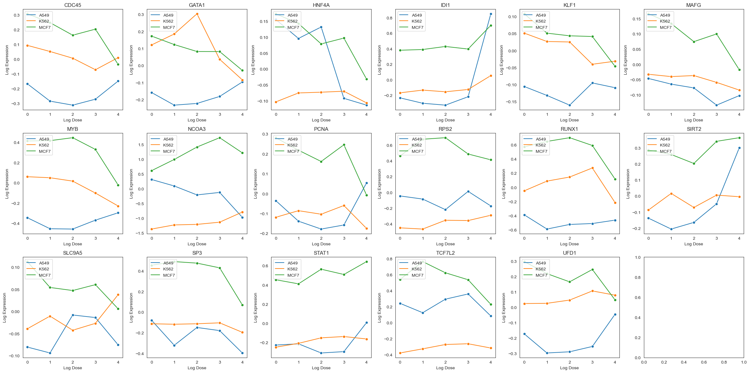
Let’s look at how each of these genes are expressed in the dataset. We plot the distribution of log expression levels for each gene, stratified by cell type and log treatment dosages. We see that the expression levels of these genes vary across cell types, and that treatment with Pracinostat (SB939) induces changes in expression levels for some genes but not others.

[23]:

def plot_average_expression(data, gene_names):
    drug_expression_df = pd.DataFrame(data[:, gene_names].layers['log1p'].toarray(), columns=gene_names)
    drug_expression_df['log10dose'] = np.log10(data.obs['dose'].values)
    drug_expression_df = drug_expression_df.replace(-np.inf, 0)
    data.obs['log10dose'] = drug_expression_df['log10dose'].values
    drug_expression_df['cell_type'] = data.obs['cell_type'].values
    avg_expression = drug_expression_df.groupby(by=['cell_type', 'log10dose']).mean().reset_index()
    avg_expression = avg_expression.melt(id_vars=['cell_type', 'log10dose'])
    avg_expression.rename({'variable': 'gene_name', 'value': 'avg_expression'}, inplace=True, axis=1)

    fig, ax = plt.subplots(3, 6, figsize=(24, 12))

    for i, gene in enumerate(gene_names):
        curr_ax = ax[i // 6][i % 6]
        if gene in avg_expression.gene_name.values:
            sns.lineplot(data=avg_expression[avg_expression.gene_name == gene],
                         x='log10dose', y='avg_expression', hue='cell_type', ax=curr_ax, marker='o')
            curr_ax.set_title(gene)
            curr_ax.set_xlabel('Log Dose')
            curr_ax.set_ylabel('Log Expression')
            curr_ax.legend(loc='upper left')
    plt.tight_layout()

We plot the average normalized gene expression levels below. These plots represent the transcriptional variation diversity from different drug dosages across different cancer cell lines. Since we do not control for any other variables, the observed correlation can be interpreted as a composition of biological signal, confounding factors, and sequencing noise. Thus, the observed correlations are not necessarily causal. In the next section, we attempt to remove the confounding factors and de-noise the sequencing data so that we can interpret the effects causally.

[24]:

plot_average_expression(drug_data, target_genes)

/var/folders/1n/rv21b_n10gx0tp5_zz33z7qc0000gn/T/ipykernel_54317/1754354712.py:3: RuntimeWarning: divide by zero encountered in log10
  drug_expression_df['log10dose'] = np.log10(data.obs['dose'].values)

Causal Probabilistic Program¶

Model Description¶

In the plots above, we did not control for technical covariates (e.g., cell plate, replicate number, etc.). Here we fit a generalized linear model with a Poission likelihood to account for the heavy-tailed count nature of the data. We also include interactions between genes and confounders (e.g., cell type, read depth, etc.) to understand how treatment effects vary across cell types and experimental conditions, and model unobserved confounders. Our model is defined as follows:

\[\begin{split}\begin{split} Z_{nk} &\sim \mathcal{N}(0, 1), \quad{1 \leq k \leq K} \quad (\text{$K$ unobserved confounders for cell}) \\ \tilde{X}_n &= (X_n, \ Z_n) \in \mathbb{R}^{p + K} \quad (\text{observed and unobserved confounders}) \\ c_g &\sim \mathcal{N}(0, 1) \quad (\text{intercept}) \\ \tau_{g} &\sim \mathcal{N}(0, 1) \quad (\text{additive treatment effect}) \\ \theta_{gi} &\sim \mathcal{N}(0, 1 / \sqrt{p + K}), \quad{1 \leq i \leq p + K} \quad (\text{additive confounder effect}) \\ \eta_{gi} &\sim \mathcal{N}(0, 1 / \sqrt{p + K}), \quad{1 \leq i \leq p + K} \quad (\text{confounder-treatment interaction effect}) \\ \log \mu_{ng} &= c_g + \tau_{g} T_n + \theta_{g}^T \tilde{X}_n + \eta_{g}^T (\tilde{X}_n \odot T_n) \quad (\text{Poisson rate}) \\ Y_{ng} &\sim \text{Poisson}(\mu_{ng}) \quad (\text{Poisson likelihood}) \\ \end{split}\end{split}\]

where $\odot$ denotes elementwise multiplication, $p$ the number of confounders, $T_n$ treatment, $X_n$ observed confounders, and $Y_{ng}$ gene expression counts for cell $n$ and gene $g$.

Note: our inclusion of the $K$ latent confounders for each cell is similar to regressing out the top principal components from the gene-expression matrix. However, our approach, which allows us to account for the uncertainty of not observing the latent confounders, is known as probabilistic principal components analysis; see Tipping (1999) for details.

[25]:

class DrugPerturbationModel(PyroModule):
    def __init__(self, num_cells: int, num_genes: int, num_observed_confounders: int, num_latent_confounders: int = 3):
        super().__init__()
        self.num_cells = num_cells
        self.num_genes = num_genes
        self.num_observed_confounders = num_observed_confounders
        self.num_latent_confounders = num_latent_confounders
        self.num_confounders = num_observed_confounders + num_latent_confounders
        self.cell_plate = pyro.plate("cells", self.num_cells, dim=-2)
        self.gene_plate = pyro.plate("genes", self.num_genes, dim=-1)

    def forward(self, mask: bool = False):
        prior_scale = 1 / math.sqrt(self.num_confounders)
        propensity_weights = pyro.sample("propensity_weights", dist.Normal(0, prior_scale).expand((self.num_confounders, )).to_event(1))

        # Sample regression weights for each gene
        with self.gene_plate:
            intercept = pyro.sample("intercept", dist.Normal(0, 1))
            theta_confounders = pyro.sample("theta_confounders", dist.Normal(0, prior_scale).expand((self.num_confounders,)).to_event(1)) # G x F
            theta_drug = pyro.sample("theta_drug", dist.Normal(0, 1))
            theta_confounders_drug = pyro.sample("theta_confounders_drug", dist.Normal(0, prior_scale).expand((self.num_confounders,)).to_event(1)) # G x F

        # Compute likelihood
        with self.cell_plate:
            # Sample treatment and confounders (remove from log_prob since we'll always conditioned on them when mask = False)
            latent_confounders = pyro.sample("latent_confounders", dist.Normal(0, 1).expand((self.num_latent_confounders,)).to_event(1))
            observed_confounders = pyro.sample("observed_confounders", dist.Normal(0, 1).expand((self.num_observed_confounders,)).mask(mask).to_event(1))
            observed_confounders = observed_confounders.expand(latent_confounders.shape[:-1] + observed_confounders.shape[-1:])
            confounders = torch.cat([observed_confounders, latent_confounders], dim=-1)  # torch.cat doesn't broadcast

            treatment_mean = torch.einsum("...ngp,...p->...ng", confounders, propensity_weights)
            T = torch.relu(pyro.sample("drug", dist.Normal(treatment_mean, 1)))
            with self.gene_plate:
                # Confounding effects
                confounder_variation = intercept + torch.einsum("...ngp,...gp->...ng", confounders, theta_confounders) # N x G

                # Drug dose treatment effects
                treatment_variation = theta_drug * T + torch.einsum("...ngp,...ng,...gp->...ng", confounders, T, theta_confounders_drug) # N x G
                mean = confounder_variation + treatment_variation # N x G
                expressions = pyro.sample("gene_expression", dist.Poisson(rate=torch.exp(mean)))
        return expressions

pyro.render_model(DrugPerturbationModel(10, 10, 10, 3), render_distributions=True, render_params=True)

[25]:

Fitting observed data¶

We further process the data for modeling by (1) one-hot encoding categorical confounders, (2) converting dosages to log dosage amounts, (3) splitting the data in training and test.

[26]:

# Restrict to top 1000 genes or those in target_genes
is_top1k_mask_or_target = sc.experimental.pp.highly_variable_genes(
    drug_data, flavor="pearson_residuals", n_top_genes=1000,
    inplace=False
)['highly_variable'].values | drug_data.var.index.isin(target_genes)

drug_data = drug_data[:, is_top1k_mask_or_target]

/opt/homebrew/anaconda3/envs/basis/lib/python3.10/site-packages/scanpy/experimental/pp/_highly_variable_genes.py:73: UserWarning: `flavor='pearson_residuals'` expects raw count data, but non-integers were found.
  warnings.warn(
/opt/homebrew/anaconda3/envs/basis/lib/python3.10/site-packages/scanpy/experimental/pp/_highly_variable_genes.py:125: RuntimeWarning: invalid value encountered in sqrt
  residuals = (X_dense - mu) / np.sqrt(mu + mu**2 / theta)

[27]:

# Make data matrices
X_confounders = pd.get_dummies(drug_data.obs[['cell_type', 'replicate', 'culture_plate', 'pcr_plate', 'well_oligo']], dtype=np.int32).reset_index(drop=True)

# Control for sequencing depth
log_umi = np.log(drug_data.obs['n.umi'].values)
scaled_log_umi = (log_umi - np.mean(log_umi)) / log_umi.std()
X_confounders['depth_proxy'] = scaled_log_umi

# For each drug, input log dose as a feature
T_all = pd.get_dummies(drug_data.obs[['product_name']], dtype=np.int32).reset_index(drop=True)
T_all = T_all.mul(np.log10(drug_data.obs['dose'].values + 1), axis=0)

# Get treatment, confounders, response for all gene expressions
X_drug_control = torch.tensor(X_confounders.values, dtype=torch.float32)
T_drug_control = torch.tensor(T_all[f'product_name_{drug_target}'].values, dtype=torch.float32)
Y_drug_control = torch.tensor(drug_data.layers['raw'].toarray(), dtype=torch.float32)

# Split into training and test set
N_drug_control = X_drug_control.shape[0]
train_mask = torch.tensor(np.random.choice([True, False], size=N_drug_control, p=[0.8, 0.2]))
X_train = X_drug_control[train_mask]
T_train = T_drug_control[train_mask]
Y_train = Y_drug_control[train_mask]
X_test = X_drug_control[~train_mask]
T_test = T_drug_control[~train_mask]
Y_test = Y_drug_control[~train_mask]

[28]:

class ConditionedDrugModel(PyroModule):
    def __init__(self, model: DrugPerturbationModel):
        super().__init__()
        self.model = model

    def forward(self, X, T, Y, **kwargs):
        with condition(data=dict(observed_confounders=X[:, None, :], drug=T[..., None], gene_expression=Y)):
            return self.model(**kwargs)

We fit our model using stochastic variational inference with a mean-field variational family.

[29]:

model_train = ConditionedDrugModel(
    DrugPerturbationModel(num_cells=Y_train.shape[0], num_genes=Y_train.shape[1], num_observed_confounders=X_train.shape[1])
)

guide_train = AutoNormal(model_train)
elbo = pyro.infer.Trace_ELBO()(model_train, guide_train)

# initialize parameters
elbo(X=X_train, T=T_train, Y=Y_train)

adam = torch.optim.Adam(elbo.parameters(), lr=0.03)

# Do gradient steps
for step in range(2000):
    adam.zero_grad()
    loss = elbo(X=X_train, T=T_train, Y=Y_train)
    loss.backward()
    adam.step()
    if step % 250 == 0:
        print("[iteration %04d] loss: %.4f" % (step, loss))

/opt/homebrew/anaconda3/envs/basis/lib/python3.10/site-packages/pyro/util.py:365: UserWarning: Found plate statements in guide but not model: {'genes', 'cells'}
  warnings.warn(

[iteration 0000] loss: 46365508.0000
[iteration 0250] loss: 3478059.2500
[iteration 0500] loss: 3372281.5000
[iteration 0750] loss: 3327728.0000
[iteration 1000] loss: 3256304.2500
[iteration 1250] loss: 3217637.2500
[iteration 1500] loss: 3223379.5000
[iteration 1750] loss: 3181398.2500

Predictions on unseen cells¶

As we see below, our predictions of gene expressions are quite poor. However, this is not very suprising because we are using a linear model, and not conditioning on more cell and gene features.

[30]:

model_test_obs = ConditionedDrugModel(
    DrugPerturbationModel(num_cells=Y_test.shape[0], num_genes=Y_test.shape[1], num_observed_confounders=X_test.shape[1])
)

guide_train.eval()
guide_test_obs = pyro.infer.autoguide.AutoGuideList(model_test_obs)
guide_test_obs.append(pyro.poutine.block(guide_train, hide=['latent_confounders', 'latent_confounders_unconstrained', 'cells', 'genes']))
guide_test_obs.append(AutoNormal(pyro.poutine.block(model_test_obs, expose=['latent_confounders', 'cells', 'genes'])))

elbo = pyro.infer.Trace_ELBO()(model_test_obs, guide_test_obs)

# initialize parameters
elbo(X=X_test, T=T_test, Y=Y_test)

adam = torch.optim.Adam(elbo.parameters(), lr=0.03)

# Do gradient steps
for step in range(2000):
    adam.zero_grad()
    loss = elbo(X=X_test, T=T_test, Y=Y_test)
    loss.backward()
    adam.step()
    if step % 250 == 0:
        print("[iteration %04d] loss: %.4f" % (step, loss))

[iteration 0000] loss: 1057932.8750
[iteration 0250] loss: 835455.9375
[iteration 0500] loss: 836271.9375
[iteration 0750] loss: 835985.6875
[iteration 1000] loss: 837112.5000
[iteration 1250] loss: 835574.3125
[iteration 1500] loss: 836130.5625
[iteration 1750] loss: 835517.8125

[31]:

predictive = pyro.infer.Predictive(model_test_obs, guide=guide_test_obs, num_samples=250)
predictive_samples = predictive(X=X_test, T=T_test, Y=None)
test_avg = predictive_samples['gene_expression'].mean(dim=0)

[42]:

# Compare posterior mean predictions across 13 genes
fig, ax = plt.subplots(3, 6, figsize=(20, 10))

for i, gene in enumerate(target_genes):
    curr_ax = ax[i // 6][i % 6]
    gene_idx = drug_data.var_names.get_loc(gene)
    curr_ax.scatter(test_avg[:, gene_idx], Y_test[:, gene_idx], alpha=0.5)
    curr_ax.set_title(gene)
    curr_ax.set_xlabel('Predicted Expression')
    curr_ax.set_ylabel('Actual Expression')

plt.tight_layout()

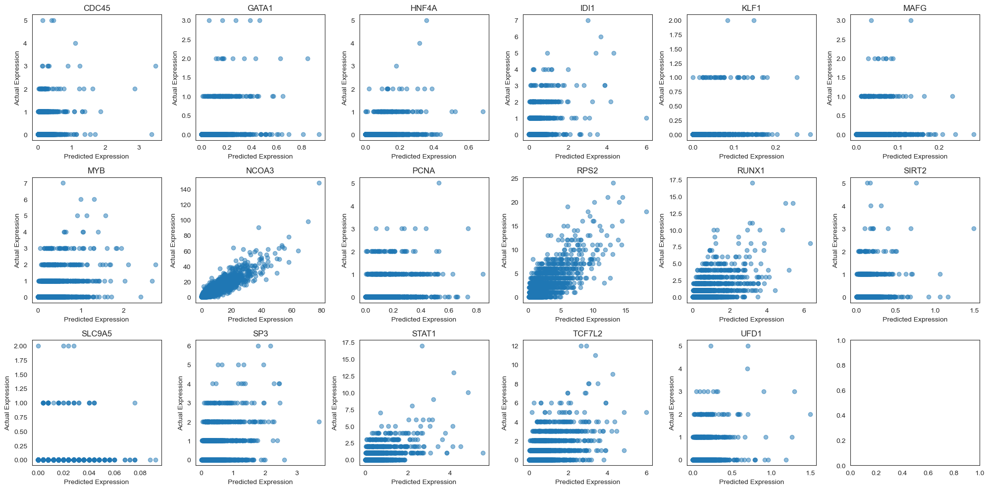
Often, we are not able to accurately predict gene expressions for individual cells. However, many papers evaluate at the bulk level instead. That is, they evaluate how well the model predicts the average expression of each gene across a collection of similar cells. We evaluate our model in this way below since it is more relevant to the downstream task of understanding the effects of a drug at the tissue level.

[43]:

# Compare posterior mean predictions across all genes
# Average gene expression comparison https://www.nature.com/articles/s41592-019-0494-8/figures/2

# Segment by cell type
fig, ax = plt.subplots(1, 3, figsize=(13, 4))
for i, cell_type in enumerate(['A549', 'MCF7', 'K562']):
    cell_type_mask = torch.tensor(drug_data[~train_mask.numpy()].obs['cell_type'].values == cell_type)
    test_avg_bulk = test_avg[cell_type_mask].mean(dim=0)

    ax[i].scatter(test_avg_bulk, Y_test[cell_type_mask].mean(dim=0), alpha=0.5)
    ax[i].set_xlabel('Average of posterior Predicted Expression across cells')
    ax[i].set_ylabel('Actual average Expression across cells')
    ax[i].set_title(f'{cell_type} Cells (Correlation={pearsonr(test_avg_bulk, Y_test[cell_type_mask].mean(dim=0))[0]:.3f})')
    ax[i].set_xscale('log')
    ax[i].set_yscale('log')
    plt.tight_layout()

Once we look at how our model performs at the bulk level, we see that the predictions are quite good.

[44]:

# Group cells by log dosage and then compare average expressions with the model
fig, ax = plt.subplots(1, 5, figsize=(20, 5))
for i, log_dose_level in enumerate([0., 1., 2., 3., 4.]):
    dose_level_mask = torch.isclose(T_test, torch.tensor(log_dose_level), atol=.2)
    test_avg_bulk = test_avg[dose_level_mask].mean(dim=0)

    ax[i].scatter(test_avg_bulk, Y_test[dose_level_mask].mean(dim=0), alpha=0.5)
    ax[i].set_xlabel('Average of posterior Predicted Expression across cells')
    ax[i].set_ylabel('Actual average Expression across cells')
    ax[i].set_title(f'Log Dosage={log_dose_level} (Correlation={pearsonr(test_avg_bulk, Y_test[dose_level_mask].mean(dim=0))[0]:.2f})')
    ax[i].set_xscale('log')
    ax[i].set_yscale('log')
plt.tight_layout()

Computing causal queries¶

For each gene in target_genes, we would like to estimate the causal effect of Pracinostat (SB939) on the gene’s expression level at each dosage level $T \in \{0, 10^1, 10^2, 10^3, 10^4\}$. Since we only observe the expression level of each cell at a particular dosage, we impute the values of the remaining dosages using our model.

Causal Query: Average treatment effect (ATE)¶

The average treatment effect summarizes, on average, how much the drug changes the expression level of a gene, $ATE(t) = \mathbb{E}[Y|do(T=t)] - \mathbb{E}[Y|do(T=0)]$. The do notation indicates that the expectations are taken according to intervened versions of the model, with $T$ set to a particular value. Note from our tutorial that this is different from conditioning on $T$ in the original causal_model, which assumes $X$ and $T$ are dependent.

In this setting, the ATE tells us how much lower or higher a gene’s expression level is when the drug is administered at a particular dosage level relative to when the drug is not administered. Here, we are interested in the average over the entire population of cells. Other estimands, such as the conditional average treatment effect, may be interested in the average effect for cells with particular attributes of interest.

To implement this query in ChiRho, we extend our DrugPerturbationModel model by applying two interventions, do(actions={"drug":0}) and do(actions={"drug": t}), and then sampling jointly from counterfactual worlds using the MultiWorldCounterfactual handler. Recall from the tutorial that the MultiWorldCounterfactual handler modifies the execution of the causal model to sample jointly from the observational and all counterfactual worlds induced by an intervention.

[45]:

class DrugPerturbationATE(pyro.nn.PyroModule):
    def __init__(self, model: DrugPerturbationModel, X_pop: torch.tensor):
        super().__init__()
        self.model = model
        # sample population confounders to average over
        self.X_pop = X_pop

    def forward(self, dose_levels: tuple):
        dose_levels = (torch.tensor(0.),) + tuple(torch.as_tensor(dose_level) for dose_level in dose_levels)

        with MultiWorldCounterfactual(), do(actions={"drug": dose_levels}), \
                condition(data=dict(observed_confounders=self.X_pop[:, None, :])):
            expressions = self.model()
            expressions_dose = gather(expressions, IndexSet(drug=set(range(2, len(dose_levels) + 1)))) # expressions predicted by model at doses > 0
            expressions_vehicle = gather(expressions, IndexSet(drug={1})) # expressions predicted by model at dose 0 (vehicle)
            return pyro.deterministic("ATEs", (expressions_dose - expressions_vehicle).mean(dim=-2))

ate_model = DrugPerturbationATE(
    DrugPerturbationModel(num_cells=Y_train.shape[0], num_genes=Y_train.shape[1], num_observed_confounders=X_train.shape[1]),
    X_pop=X_train
)
ate_predictive = pyro.infer.Predictive(ate_model, guide=guide_train, num_samples=250, return_sites=("ATEs",))

log_dose_levels = (1., 2., 3., 4.)
ate_samples = ate_predictive(log_dose_levels)['ATEs'].squeeze()

[46]:

# Issues w/ shuffling
target_mask_reindexed = drug_data.var.index.isin(target_genes)
target_genes_reindexed = drug_data.var.index[target_mask_reindexed]

[47]:

fig, ax = plt.subplots(2, 2, figsize=(15, 8))

for i, dose_level in enumerate(log_dose_levels):
    curr_ax = ax[i // 2][i % 2]
    sns.boxplot(pd.DataFrame(ate_samples[:, i, target_mask_reindexed], columns=target_genes_reindexed), color='green', ax=curr_ax)
    curr_ax.set_title(f'Average Treatment Effect (Dosage = $10^{int(dose_level)}$)')
    curr_ax.axhline(0, color='black', linestyle='--', label='Zero treatment effect')
    curr_ax.set_xlabel('Target Gene')
    for tick in curr_ax.get_xticklabels():
        tick.set_rotation(45)
    curr_ax.set_ylabel('Average Treatment Effect')
    curr_ax.legend()
    curr_ax.set_ylim(-.5, .5)
    sns.despine()

plt.tight_layout()

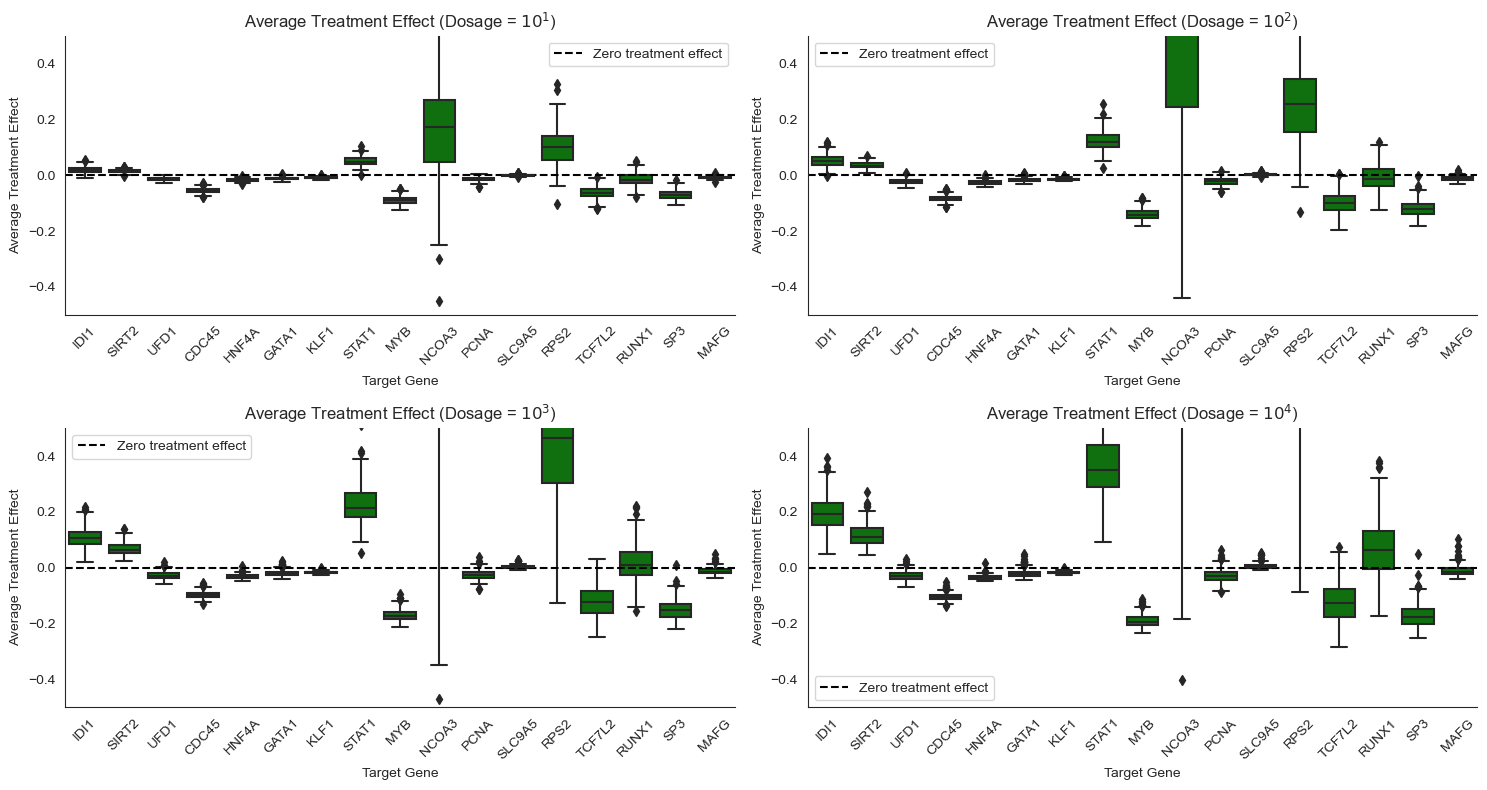
The plot above provides the uncertainity across the average treatment effect for each gene. The upper (75th%) and lower lines (25th%) on each boxplot form a 50% credible interval for the average treatment effect by gene, cell type, and dosage. The positive effect on SIRT2, which deacetylates tubulin, is consistent with the conclusion from Srivatsan (2020). This phenomenon, also known as genetic compensation response (GCR), is a mechanism to maintain the robustness of redundant functional genes and a survival strategy for cancer and microbiology (Xu 2023, El-Brolosy 2017). It also forms the therapeutic basis for targeting synthetic lethal genes in the same pathway or as paralogs (Ryan 2023).

Causal Query: Conditional average treatment effect (CATE)¶

The ATE summarizes how much the drug changes the expression level of a gene on average, but certain types of cells might respond differently to the drug. In this setting we wish to compute the conditional average treatment effect, $CATE(t) = \mathbb{E}[Y|do(T=t), X=x] - \mathbb{E}[Y|do(T=0), X=x]$, which controls for cell-specific confounders $X$.

In words, in this setting the CATE tells us how much lower or higher a gene’s expression level is when the drug is administered at a particular dosage level relative to when the drug is not administered, for cells with the same set of confounders. Here, we are interested in the average only over that subpopulation of cells with the same value of the confounders.

[48]:

class DrugPerturbationCATE(pyro.nn.PyroModule):
    def __init__(self, model: DrugPerturbationModel):
        super().__init__()
        self.model = model

    def forward(self, dose_levels: tuple, X: torch.tensor, T: torch.tensor, Y: torch.tensor):
        dose_levels = (torch.tensor(0.),) + tuple(torch.as_tensor(dose_level) for dose_level in dose_levels)

        with MultiWorldCounterfactual(), do(actions={"drug": dose_levels}), \
                condition(data={"observed_confounders": X[:, None, :], "drug": T[..., None], "gene_expression": Y}):
            expressions = self.model()
            expressions_dose = gather(expressions, IndexSet(drug=set(range(2, len(dose_levels) + 1)))) # expressions predicted by model at doses > 0
            expressions_vehicle = gather(expressions, IndexSet(drug={1})) # expressions predicted by model at dose 0 (vehicle)
            return pyro.deterministic("CATEs", (expressions_dose - expressions_vehicle))

[49]:

log_dose_levels = (1., 2., 3., 4.)
cell_types = ['A549', 'MCF7', 'K562']

# Conditional average treatment effect for each cell
cate_model = DrugPerturbationCATE(
        DrugPerturbationModel(num_cells=X_test.shape[0], num_genes=Y_test.shape[1], num_observed_confounders=X_test.shape[1])
    )

cate_predictive = pyro.infer.Predictive(cate_model, guide=guide_test_obs, num_samples=250, return_sites=("CATEs",))
cate_for_each_cell = cate_predictive(log_dose_levels, X_test, T_test, Y_test)['CATEs'].squeeze()

# To get conditional average treatment by cell type, we average cate_predictive across the subset of cells that are of each cell type
cate_samples = {}
for cell_type in cell_types:
    cell_type_mask = torch.tensor(drug_data.obs['cell_type'].values == cell_type)[~train_mask]

    # condition on cell type, average over other covariates by averaging over cells
    # cate_samples is matrix of size num posterior samples x num dosages x num cells x num genes
    cate_samples[cell_type] = cate_for_each_cell[:, :, cell_type_mask, :].mean(dim=-2)

[50]:

for cell_type in cell_types:
    fig, ax = plt.subplots(2, 2, figsize=(15, 8))

    for i, dose_level in enumerate(log_dose_levels):
        curr_ax = ax[i // 2][i % 2]
        sns.boxplot(pd.DataFrame(cate_samples[cell_type][:, i, target_mask_reindexed], columns=target_genes_reindexed), color='green', ax=curr_ax)
        curr_ax.set_title(f'Conditional Average Treatment Effect (Cell Type = {cell_type}, Dosage = $10^{int(dose_level)}$)')
        curr_ax.axhline(0, color='black', linestyle='--', label='Zero treatment effect')
        curr_ax.set_xlabel('Target Gene')
        for tick in curr_ax.get_xticklabels():
            tick.set_rotation(45)
        curr_ax.set_ylabel('Cell Type Conditional Average Treatment Effect')
        curr_ax.set_ylim(-.5, .5)
        curr_ax.legend()
        sns.despine()

    plt.tight_layout()

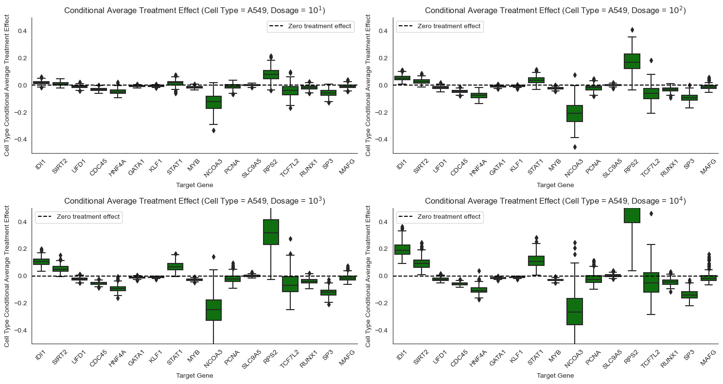
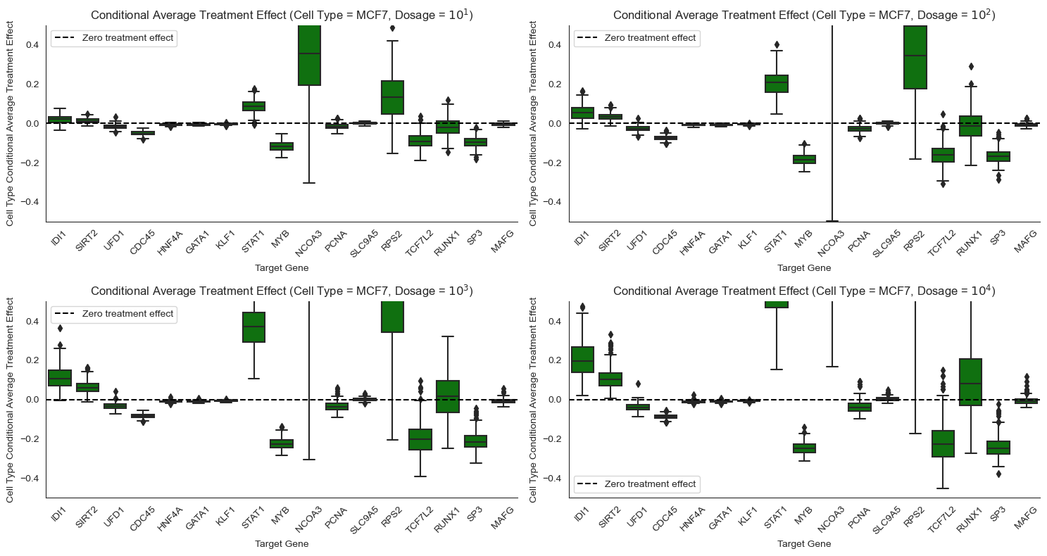
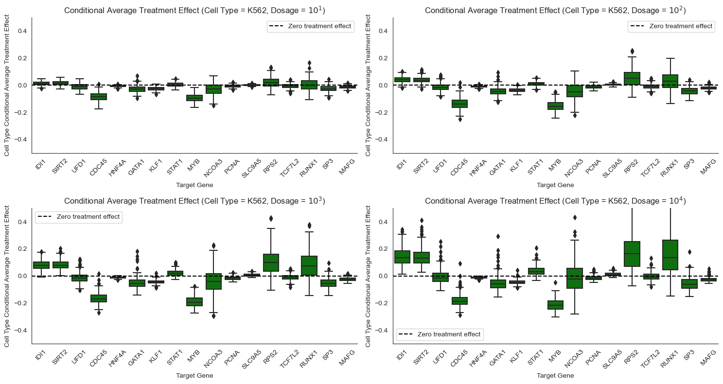
Some genes respond differently to Pracinostat (SB939) depending on cell type. For example, STAT1 responds more strongly to Pracinostat (SB939) in MCF7 cells than in K562 cells. NCOA3 shows extremely high positive effect for MCF7 but a significant negative effect for A549, and weak negative effect for K562. Such heterogeneity motivates the need for personalized medicine, where different drugs are designed for different patient genomes.

Other genes respond similarly to Pracinostat (SB939) across cell types. For example, STAT1 and IDI1 exhibit minor to significant treatment effects for all the cancer cell lines. Similarly, RP52, a housekeeping gene, has consistent effects across cell types. Hence, there might be a generic drug that works for many different patients in certain instances.

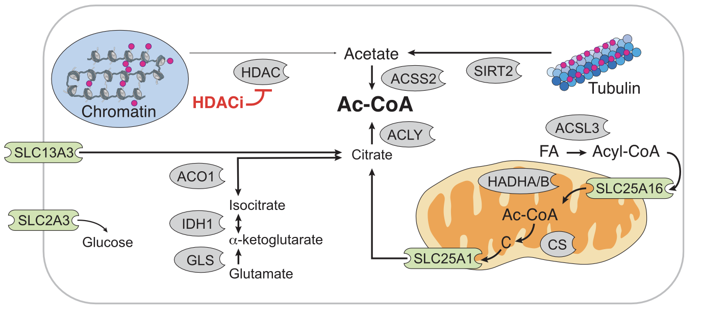
We conclude by showing Figure 5B from Srivatsan (2020) below. This figure shows how HDAC inhibitors such as Pracinostat (SB939) affect the expression of other genes such as SIRT2. Our findings above for SIRT2 validate the findings in Srivatsan (2020), where the authors also state that HDAC inhibitors such as Pracinostat (SB939) upregulate SIRT2.

[51]:

# Figure 5B from Srivatsan (2020)
# Diagram of the roles of genes from (A) in cytoplasmic acetyl-CoA regulation.
# Red circles indicate acetyl groups. Enzymes are shown in gray. Transporters are shown in green
# (FA, fatty acid; Ac-CoA, acetyl-CoA; C, citrate).
Image('./figures/sciplex_fig5b.png', width=700)

[51]:

References¶

Sanjay R., Srivatsan et al., “Massively multiplex chemical transcriptomics at single-cell resolution”. Science, 2020. https://www.science.org/doi/10.1126/science.aax6234

Hyun-Jung Kim, Suk-Chul Bae. “Histone deacetylase inhibitors: molecular mechanisms of action and clinical trials as anti-cancer drugs”. American Journal of Translational Research, 2011. https://www.ncbi.nlm.nih.gov/pmc/articles/PMC3056563/

Guo Li, Yuan Tian, Wei-Guo Zhu. “The Roles of Histone Deacetylases and Their Inhibitors in Cancer Therapy”. Frontiers in Cell and Developmental Biology, 2020. https://www.frontiersin.org/articles/10.3389/fcell.2020.576946/full

Daryl C. Drummond et al. “Clinical development of histone deacetylase inhibitors as anticancer agents”. Annual Review of Pharmacology and Toxicology, 2005. https://www.annualreviews.org/doi/10.1146/annurev.pharmtox.45.120403.095825.

Xiang-Jiao Yang, Edward Seto. “HATs and HDACs: from structure, function and regulation to novel strategies for therapy and prevention”. Oncogene, 2007. https://www.nature.com/articles/1210599.

Mohamed A. El-Brolosy, Didier Y. R. Stainier. “Genetic compensation: A phenomenon in search of mechanisms”. PLOS Genetics, 2017. https://journals.plos.org/plosgenetics/article?id=10.1371/journal.pgen.1006780.

Weimin Xu, Weijun Ou, Yuan Feng, Qingru Xu, Yili Yang, Long Cui, Peng Du. “Genetic compensation response could exist in colorectal cancer: UPF3A upregulates the oncogenic homologue gene SRSF3 expression corresponding to SRSF6 to promote colorectal cancer metastasis”. Journal of Gastroenterology and Hepatology, 2023. https://onlinelibrary.wiley.com/doi/full/10.1111/jgh.16152

Colm J. Ryan, Ishan Mehta, Narod Kebabci, David J. Adams. “Targeting synthetic lethal paralogs in cancer”. Trends in Cancer, 2023. https://www.cell.com/trends/cancer/fulltext/S2405-8033(23)00022-5

Michael E. Tipping, Christopher M. Bishop. “Probabilistic principal component analysis”. Journal of Royal Statistical Society B, 1999. https://rss.onlinelibrary.wiley.com/doi/abs/10.1111/1467-9868.00196